nlhwPlot
Plot input and output nonlinearity, and linear responses of Hammerstein-Wiener model
Since R2023a
Syntax
Description
nlhwPlot( plots the input and output
nonlinearity, and linear responses of a Hammerstein-Wiener model on a Hammerstein-Wiener
plot. The plot shows the responses of the input and output
nonlinearity, and linear blocks that represent the model.model)
nlhwPlot(model1,...,modelN) generates the plot for multiple
models.
nlhwPlot(model1,LineSpec1...,modelN,LineSpecN) specifies the line style
for each model. You do not need to specify the line style for all models.
nlhwPlot(___, specifies plot
properties using additional options specified by one or more
Name,Value)Name,Value pair arguments. This syntax can include any
of the input argument combinations in the previous syntaxes.
Examples
Estimate a Hammerstein-Wiener Model and plot responses of its input and output nonlinearity and linear blocks.
load mrdamper V F Ts
model = nlhw(V(1:500),F(1:500),[2 2 1],idSigmoidNetwork(2),idGaussianProcess('Matern32'),Ts=Ts);
nlhwPlot(model)
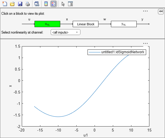
Explore the various plots in the plot window by clicking one of the three blocks that represent the model:
uNL - Input nonlinearity, representing the static nonlinearity at the input (
model.InputNonlinearity) to the Linear Block.Linear Block - Step, impulse,Bode and pole-zero plots of the embedded linear model (
model.LinearModel). By default, a step plot is displayed.yNL - Output nonlinearity, representing the static nonlinearity at the output (
model.OutputNonlinearity) of the Linear Block.
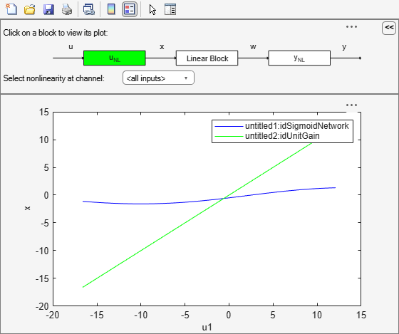
load mrdamper V F Ts
model1 = nlhw(V(1:500),F(1:500),[2 2 1],idSigmoidNetwork(2),idGaussianProcess('Matern32'),Ts=Ts)
model1 =

Hammerstein-Wiener model with 1 output and 1 input

Linear transfer function corresponding to the orders nb = 2, nf = 2, nk = 1

Input nonlinearity: Sigmoid network with 2 units
Output nonlinearity: Gaussian process function using a Matern32 kernel
Sample time: 0.005 seconds

Status:
Estimated using NLHW on time domain data.
Fit to estimation data: 85.73%
FPE: 68.22, MSE: 64.25

Model Properties
model2 = nlhw(V(1:500),F(1:500),[2 2 1],[],'idSigmoidNetwork',Ts=Ts);
nlhwPlot(model1,'b-',model2,'g')
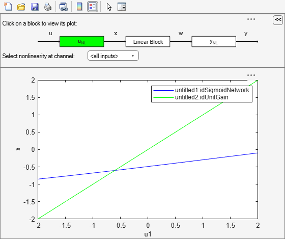
load mrdamper V F Ts
model1 = nlhw(V(1:500),F(1:500),[2 2 1],idSigmoidNetwork(2),idGaussianProcess('Matern32'),Ts=Ts);
model2 = nlhw(V(1:500),F(1:500), [2 2 1],[],'idSigmoidNetwork',Ts=Ts);
nlhwPlot(model1,'b-',model2,'g','NumberOfSamples',50,'time',10,'InputRange',[-2 2]);
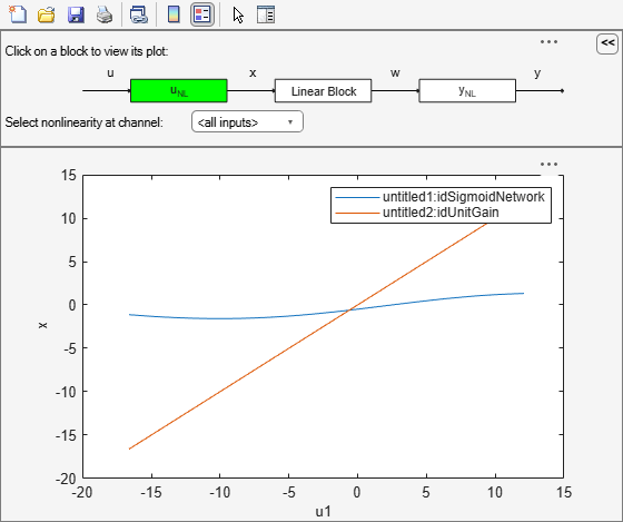
load mrdamper V F Ts
model1 = nlhw(V(1:500),F(1:500),[2 2 1],idSigmoidNetwork(2),idGaussianProcess('Matern32'),Ts=Ts);
model2 = nlhw(V(1:500),F(1:500),[2 2 1],[],'idSigmoidNetwork',Ts=Ts);
nlhwPlot(model1,model2,'time',1:500,'freq',{0.01,100},'OutputRange',[0 1000]);
Input Arguments
Name-Value Arguments
More About
A Hammerstein-Wiener plot displays the static input and output nonlinearities and linear responses of a Hammerstein-Wiener model.
Examining a Hammerstein-Wiener plot can help you determine whether you have selected a complicated nonlinearity for modeling your system. For example, suppose you use a piecewise-linear input nonlinearity to estimate your model, but the plot indicates saturation behavior. You can estimate a new model using the simpler saturation nonlinearity instead. For multivariable systems, you can use the Hammerstein-Wiener plot to determine whether to exclude nonlinearities for specific channels. If the nonlinearity for a specific input or output channel does not exhibit strong nonlinear behavior, you can estimate a new model after setting the nonlinearity at that channel to unit gain.
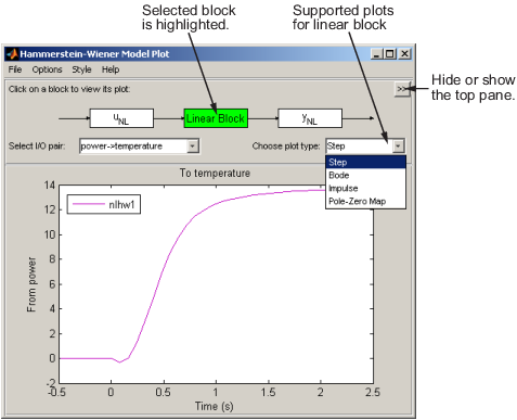
You can generate these plots in the System Identification app and at the command line. In the plot window, you can view the nonlinearities and linear responses by clicking one of the three blocks that represent the model:
uNL (input nonlinearity)— Click this block to view the static nonlinearity at the input to the
Linear Block. The plot displaysevaluate(M.InputNonlinearity,u)whereMis the Hammerstein-Wiener model, anduis the input to the input nonlinearity block. For information about the blocks, see Structure of Hammerstein-Wiener Models.Linear Block— Click this block to view the Step, impulse, Bode, and pole-zero response plots of the embedded linear model (M.LinearModel). By default, a step plot of the linear model is displayed.yNL (output nonlinearity) — Click this block to view the static nonlinearity at the output of the
Linear Block. The plot displaysevaluate(M.OutputNonlinearity,x), wherexis the output of the linear block.
To learn more about how to configure the linear and nonlinear blocks plots, see Configuring a Hammerstein-Wiener Plot.