Heat Exchanger (TL)
Heat exchanger for systems with thermal liquid and controlled flows
Libraries:
Simscape /
Fluids /
Heat Exchangers /
Thermal Liquid
Description
The Heat Exchanger (TL) block models the cooling and heating of fluids through conduction over a thin wall. The properties of a single-phase thermal liquid are defined on the Thermal Liquid tab. The second fluid is a controlled fluid, which is specified only by the user-defined parameters on the Controlled Fluid tab. It does not receive any properties from the domain fluid network. The heat exchange between the fluids is based on the thermal liquid sensible heat.
Heat Transfer Model
The block heat transfer model derives from the Effectiveness-NTU method. The steady-state heat transfer is determined based on a coefficient relating ideal to real losses in the system:
where
Q the actual heat transfer rate.
QMax is the ideal heat transfer rate.
ε is the heat exchanger effectiveness, which is based on the ratio of heat capacity rates, , and the exchanger Number of Transfer Units:
where R is the overall thermal resistance, which is discussed in Thermal Resistance below. CMin is the lesser heat capacity rate of the two fluids and CMax is the greater heat capacity rate of the two fluids. The heat capacity rate is calculated as
Additionally, the exchanger effectiveness depends on the number of passes between the fluids and the fluid mixing conditions. For a list of the effectiveness expressions, see the E-NTU Heat Transfer block. Connect an E-NTU Heat Transfer block to a Heat Exchanger (TL) block to specify the heat transfer properties in with the E-NTU method.
The fluid properties that the block uses in heat transfer calculations are the average between the value at the inlet and the value in the fluid volume.
Flow Arrangement
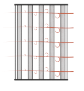
Use the Flow arrangement parameter to define the flow configuration in terms of pipe orientation or effectiveness tables. When using the shell-and-tube configuration, you can select the number of passes in the exchanger. A multi-pass exchanger resembles the image below.
A single-pass exchanger resembles the image below.
Other flow arrangements are possible through a generic parameterization by tabulated effectiveness data. This table does not require specific heat exchanger configuration details, such as flow arrangement, mixing, and passes, for modeling the heat transfer between the fluids.
Mixing Condition
Use the Cross flow type parameter to model flows that are not restricted by baffles or walls, which homogenizes fluid temperature along the direction of flow of the second fluid and varies perpendicular to the second fluid flow. Unmixed flows vary in temperature both along and perpendicular to the flow direction of the second fluid. An example of a heat exchanger with one mixed and one unmixed fluid resembles the configuration below.
A heat exchanger with two unmixed fluids resembles the configuration below.

In counter and parallel flow arrangements, longitudinal temperature variation in one fluid results in a longitudinal change in temperature variation in the second fluid and mixing is not taken into account.
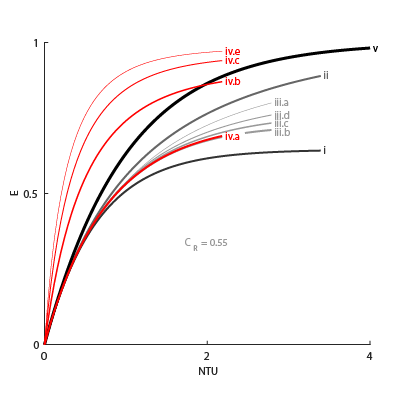
Effectiveness Curves
Shell-and-tube exchangers with multiple passes (iv.b-e in the figure for 2, 3, and 4 passes) are the most effective type of heat exchanger. For single-pass heat exchangers, the counter-flow configuration (ii) is the most effective, and parallel flow (i) is the least.
Cross-flow exchangers are intermediate in effectiveness, with mixing condition playing a factor. They are most effective when both flows are unmixed (iii.a) and least effective when both flows are mixed (iii.b). Mixing just the flow with the smallest heat capacity rate (iii.c) lowers the effectiveness more than mixing just the flow with the largest heat capacity rate (iii.d).
Thermal Resistance
The overall thermal resistance, R, is the sum of the local resistances to heat transfer due to convection, conduction, and fouling along the heat exchanger walls.
where:
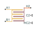
U1 is the heat transfer coefficient between the thermal liquid and the wall.
U2 is the heat transfer coefficient between the controlled fluid and the wall, which is received as a physical signal at port HC2.
F1 is the thermal liquid Fouling factor.
F2 is the controlled fluid Fouling factor.
A1 is the thermal liquid Heat transfer surface area.
A2 is the controlled fluid Heat transfer surface area.
RW is the Wall thermal resistance.
The heat transfer coefficients depend on the heat exchanger configuration and fluid properties. See the E-NTU Heat Transfer reference page for more information.
Wall Thermal Mass
If you select Enable wall thermal mass, the block models the heat exchanger wall thermal mass, which introduces a delay in the wall's transient response to changes in temperature or heat flux. If you model thermal mass, the wall stores heat in its bounds. This heat storage slows the transition between steady states so that a thermal perturbation on one side does not immediately manifest on the other side. The lag persists until the heat flow rates from the two sides balance.
If you select Enable wall thermal mass, the wall energy conservation is
where:
Mwall is the value of the Wall mass parameter.
cp,wall is the value of the Wall specific heat parameter.
Twall is the effective wall temperature on each side. The block uses this value to model the transient response. You cannot measure this value.
The heat transfer to each fluid is
where:
Tin is the fluid inlet temperature on each side.
C is the heat capacity rate for each fluid.
The number of heat transfer units between the fluid and the wall on each side is
where A is the wall surface area and U is the heat transfer coefficient.
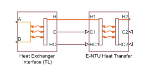
Composite Structure
When the Heat Exchanger (TL) block is a composite of the Heat Exchanger Interface (TL) and E-NTU Heat Transfer blocks:
Examples

Engine Cooling System
Model an engine cooling system with an oil cooling circuit.

House Heating System
Model a simple house heating system. The model contains a heater, a controller, and a house structure with four radiators and four rooms. Each room exchanges heat with the environment through its exterior walls, roof, and windows. Each path is simulated as a combination of a thermal convection, thermal conduction, and the thermal mass. It is assumed that heat is not transferred internally between rooms. The heater consists of a furnace, a boiler, an accumulator, and a pump to circulate hot water in the system. The controller starts admitting fuel into the furnace if the overall average temperature of rooms falls below 21 degree C and it stops if the temperature exceeds 25 degree C. The simulation calculates the heating cost and indoor temperatures.

Hydraulic Oil System with Thermal Control
A hydraulic oil system with a thermal control using Simscape™ Fluids™ Thermal Liquid blocks. The hydraulic oil system consists of an oil storage tank represented by the Tank (TL) block with two inlets, a pump represented by a Mass Flow Rate Source (TL) block, and pipelines represented by Pipe (TL) block.