このページは機械翻訳を使用して翻訳されました。最新版の英語を参照するには、ここをクリックします。
粒子群出力関数
この例では、particleswarm の出力関数を使用する方法を示します。出力関数は、各次元で粒子が占める範囲をプロットします。
出力関数は、ソルバーの各反復後に実行されます。構文の詳細と出力関数で使用できるデータについては、出力関数とプロット関数 を参照してください。
カスタムプロット関数
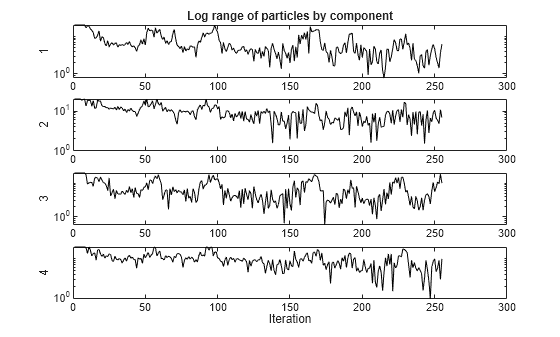
この例の最後にある pswplotranges ヘルパー関数は、次元ごとに 1 本の線でプロットを描画します。各線は、その次元における群れの中の粒子の範囲を表します。プロットは、広い範囲に対応するために対数スケールになっています。群れが単一の点に収束すると、各次元の範囲はゼロになります。しかし、群れが一点に収束しない場合は、いくつかの次元で範囲はゼロから離れた状態になります。
目的関数
この例の最後にある multirosenbrock ヘルパー関数は、Rosenbrock 関数を任意の偶数次元に一般化します。[1,1,1,1,...] の点では 0 が大域的最小値となります。
セットアップと実行の問題
multirosenbrock 関数を目的関数として設定します。4 つの変数を使用します。各変数に下限値 -10 と上限値 10 を設定します。
fun = @multirosenbrock;
nvar = 4; % A 4-D problem
lb = -10*ones(nvar,1); % Bounds to help the solver converge
ub = -lb;
出力関数を使用するためのオプションを設定します。
options = optimoptions(@particleswarm,'OutputFcn',@pswplotranges);再現可能な結果を得るには、乱数ジェネレーターを設定します。次にソルバーを呼び出します。
rng default % For reproducibility
[x,fval,eflag] = particleswarm(fun,nvar,lb,ub,options)
Optimization ended: relative change in the objective value
over the last OPTIONS.MaxStallIterations iterations is less than OPTIONS.FunctionTolerance.
x = 1×4

    0.9964    0.9930    0.9835    0.9681
fval =
3.4935e-04
eflag =
1
結果
ソルバーは最適な [1,1,1,1] に近い点を返します。しかし、群れの範囲はゼロに収束しません。
補助関数
次のコードは、pswplotranges 補助関数を作成します。
function stop = pswplotranges(optimValues,state)

stop = false; % This function does not stop the solver
switch state
    case 'init'
        fig = figure();
        set(fig,'numbertitle','off','name','pranges')
        nplot = size(optimValues.swarm,2); % Number of dimensions
        for i = 1:nplot % Set up axes for plot
            subplot(nplot,1,i);
            tag = sprintf('psoplotrange_var_%g',i); % Set a tag for the subplot
            semilogy(optimValues.iteration,0,'-k','Tag',tag); % Log-scaled plot
            ylabel(num2str(i))
        end
        xlabel('Iteration','interp','none'); % Iteration number at the bottom
        subplot(nplot,1,1) % Title at the top
        title('Log range of particles by component')
        setappdata(gcf,'t0',tic); % Set up a timer to plot only when needed
    case 'iter'
        fig = findobj(0,'Type','figure','Name','pranges');
        set(0,'CurrentFigure',fig);
        nplot = size(optimValues.swarm,2); % Number of dimensions
        for i = 1:nplot
            subplot(nplot,1,i);
            % Calculate the range of the particles at dimension i
            irange = max(optimValues.swarm(:,i)) - min(optimValues.swarm(:,i));
            tag = sprintf('psoplotrange_var_%g',i);
            plotHandle = findobj(get(gca,'Children'),'Tag',tag); % Get the subplot
            xdata = plotHandle.XData; % Get the X data from the plot
            newX = [xdata optimValues.iteration]; % Add the new iteration
            plotHandle.XData = newX; % Put the X data into the plot
            ydata = plotHandle.YData; % Get the Y data from the plot
            newY = [ydata irange]; % Add the new value
            plotHandle.YData = newY; % Put the Y data into the plot
        end
        if toc(getappdata(gcf,'t0')) > 1/30 % If 1/30 s has passed
          drawnow % Show the plot
          setappdata(gcf,'t0',tic); % Reset the timer
        end
    case 'done'
        % No cleanup necessary
end
end
次のコードは、multirosenbrock 補助関数を作成します。
function F = multirosenbrock(x)
% This function is a multidimensional generalization of Rosenbrock's
% function. It operates in a vectorized manner, assuming that x is a matrix
% whose rows are the individuals.

% Copyright 2014 by The MathWorks, Inc.

N = size(x,2); % assumes x is a row vector or 2-D matrix
if mod(N,2) % if N is odd
    error('Input rows must have an even number of elements')
end

odds  = 1:2:N-1;
evens = 2:2:N;
F = zeros(size(x));
F(:,odds)  = 1-x(:,odds);
F(:,evens) = 10*(x(:,evens)-x(:,odds).^2);
F = sum(F.^2,2);
end