このページは機械翻訳を使用して翻訳されました。最新版の英語を参照するには、ここをクリックします。
GlobalSearch および MultiStart を使用した単色偏光干渉パターンの最大化
この例では、関数 GlobalSearch と MultiStart の使用方法を示します。
はじめに
この例では、Global Optimization Toolbox 関数、特に GlobalSearch と MultiStart が、電磁干渉パターンの最大値を見つけるのにどのように役立つかを示します。モデル化を簡単にするために、パターンは点光源から広がる単色偏光から生じます。
点xと時刻tで分極方向に測定されたソースiによる電界は
![]()
ここで、![]() はソース
はソース ![]() の時間ゼロでの位相、
の時間ゼロでの位相、![]() は光速、
は光速、![]() は光の周波数、
は光の周波数、![]() はソース
はソース ![]() の振幅、
の振幅、![]() はソース
はソース ![]() から
から ![]() までの距離です。
までの距離です。
固定点 ![]() の場合、光の強度は正味電場の 2 乗の時間平均です。正味電界は、すべての発生源による電界の合計です。時間平均は、
の場合、光の強度は正味電場の 2 乗の時間平均です。正味電界は、すべての発生源による電界の合計です。時間平均は、![]() における電界の大きさと相対位相にのみ依存します。正味電界を計算するには、位相器法を使用して個体の寄与を合計します。位相器の場合、各ソースはベクトルを提供します。ベクトルの長さは振幅を音源からの距離で割った値であり、ベクトルの角度
における電界の大きさと相対位相にのみ依存します。正味電界を計算するには、位相器法を使用して個体の寄与を合計します。位相器の場合、各ソースはベクトルを提供します。ベクトルの長さは振幅を音源からの距離で割った値であり、ベクトルの角度 ![]() はその点における位相です。
はその点における位相です。
この例では、周波数 (![]() ) と振幅 (
) と振幅 (![]() ) が同じで、初期位相 (
) が同じで、初期位相 (![]() ) が異なる 3 つの点音源を定義します。これらのソースを固定された平面上に配置します。
) が異なる 3 つの点音源を定義します。これらのソースを固定された平面上に配置します。
% Frequency is proportional to the number of peaks
relFreqConst = 2*pi*2.5;
amp = 2.2;
phase = -[0; 0.54; 2.07];

numSources = 3;
height = 3;

% All point sources are aligned at [x_i,y_i,z]
xcoords = [2.4112
           0.2064
           1.6787];
ycoords = [0.3957
           0.3927
           0.9877];
zcoords = height*ones(numSources,1);

origins = [xcoords ycoords zcoords];
干渉パターンを視覚化する
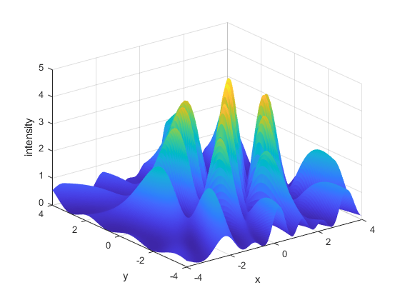
ここで、平面 z = 0 上の干渉パターンのスライスを視覚化してみましょう。
下のグラフからわかるように、建設的干渉と破壊的干渉を示す山と谷が多数あります。
% Pass additional parameters via an anonymous function:
waveIntensity_x = @(x) waveIntensity(x,amp,phase, ...
    relFreqConst,numSources,origins);
% Generate the grid
[X,Y] = meshgrid(-4:0.035:4,-4:0.035:4);
% Compute the intensity over the grid
Z = arrayfun(@(x,y) waveIntensity_x([x y]),X,Y);
% Plot the surface and the contours
figure
surf(X,Y,Z,'EdgeColor','none')
xlabel('x')
ylabel('y')
zlabel('intensity')
最適化問題の提起
私たちが興味を持っているのは、この波の強度が最高に達する場所です。
波の強度 (![]() ) は、発生源から離れるにつれて、
) は、発生源から離れるにつれて、![]() に比例して減少します。したがって、問題に制約を追加して、実行可能なソリューションの空間を制限しましょう。
に比例して減少します。したがって、問題に制約を追加して、実行可能なソリューションの空間を制限しましょう。
開口部で光源の露出を制限すると、開口部の投影が観測面に交差する部分に最大値が存在することが予想されます。各ソースを中心とした円形領域に探索を制限することで、開口部の効果をモデル化します。
また、問題に境界を追加することで、解空間を制限します。これらの境界は冗長になる可能性がありますが (非線形制約を考慮すると)、開始点が生成される範囲を制限するので便利です (詳細については、GlobalSearchとMultiStartの仕組み を参照してください)。
今、私たちの問題は次のようになりました:
![]()
制約条件
![]()
![]()
![]()
![]()
![]()
ここで、![]() と
と ![]() は、それぞれ
は、それぞれ ![]() 点光源の座標と開口半径です。各光源には半径 3 の開口部が与えられます。指定された境界は実行可能な領域を囲みます。
点光源の座標と開口半径です。各光源には半径 3 の開口部が与えられます。指定された境界は実行可能な領域を囲みます。
目的関数 (![]() ) と非線形制約関数は、それぞれ別の MATLAB ® ファイル、
) と非線形制約関数は、それぞれ別の MATLAB ® ファイル、waveIntensity.m と apertureConstraint.m で定義されており、この例の最後にリストされています。
制約付きの可視化
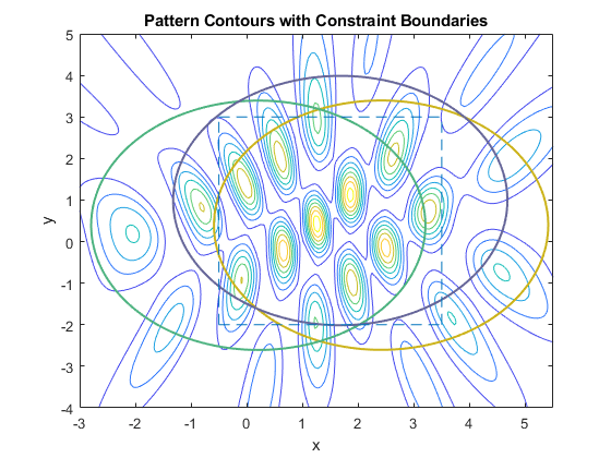
ここで、非線形制約境界を重ね合わせた干渉パターンの輪郭を視覚化してみましょう。実現可能領域は、3 つの円 (黄色、緑、青) の交点の内側です。変数の境界は破線のボックスで示されます。
% Visualize the contours of our interference surface
domain = [-3 5.5 -4 5];
figure;
ezcontour(@(X,Y) arrayfun(@(x,y) waveIntensity_x([x y]),X,Y),domain,150);
hold on

% Plot constraints
g1 = @(x,y)  (x-xcoords(1)).^2 + (y-ycoords(1)).^2 - 9;
g2 = @(x,y)  (x-xcoords(2)).^2 + (y-ycoords(2)).^2 - 9;
g3 = @(x,y)  (x-xcoords(3)).^2 + (y-ycoords(3)).^2 - 9;
h1 = ezplot(g1,domain);
h1.Color = [0.8 0.7 0.1]; % yellow
h1.LineWidth = 1.5;
h2 = ezplot(g2,domain);
h2.Color = [0.3 0.7 0.5]; % green
h2.LineWidth = 1.5;
h3 = ezplot(g3,domain);
h3.Color = [0.4 0.4 0.6]; % blue
h3.LineWidth = 1.5;

% Plot bounds
lb = [-0.5 -2];
ub = [3.5 3];
line([lb(1) lb(1)],[lb(2) ub(2)],'LineStyle','--')
line([ub(1) ub(1)],[lb(2) ub(2)],'LineStyle','--')
line([lb(1) ub(1)],[lb(2) lb(2)],'LineStyle','--')
line([lb(1) ub(1)],[ub(2) ub(2)],'LineStyle','--')
title('Pattern Contours with Constraint Boundaries')
ローカルソルバーによる問題の設定と解決
非線形制約が与えられた場合、制約付き非線形ソルバー、つまり fmincon が必要になります。
最適化の問題を記述する問題構造を設定しましょう。強度関数を最大化したいので、waveIntensity から返される値を否定します。実行可能領域に近い任意の開始点を選択しましょう。
この小さな問題では、fmincon の SQP アルゴリズムを使用します。
% Pass additional parameters via an anonymous function:
apertureConstraint_x = @(x) apertureConstraint(x,xcoords,ycoords);

% Set up fmincon's options
x0 = [3 -1];
opts = optimoptions('fmincon','Algorithm','sqp');
problem = createOptimProblem('fmincon','objective', ...
    @(x) -waveIntensity_x(x),'x0',x0,'lb',lb,'ub',ub, ...
    'nonlcon',apertureConstraint_x,'options',opts);

% Call fmincon
[xlocal,fvallocal] = fmincon(problem)
Local minimum found that satisfies the constraints.

Optimization completed because the objective function is non-decreasing in
feasible directions, to within the value of the optimality tolerance,
and constraints are satisfied to within the value of the constraint tolerance.


xlocal =

   -0.5000    0.4945


fvallocal =

   -1.4438
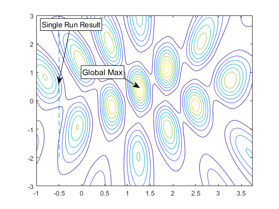
ここで、等高線図で fmincon の結果を表示して、結果を確認してみましょう。fmincon はグローバル最大値に到達しなかったことに注意してください。これはプロットにも注釈が付けられています。解において有効であった境界のみをプロットすることに注意してください。
[~,maxIdx] = max(Z(:));
xmax = [X(maxIdx),Y(maxIdx)]
figure
contour(X,Y,Z)
hold on

% Show bounds
line([lb(1) lb(1)],[lb(2) ub(2)],'LineStyle','--')

% Create textarrow showing the location of xlocal
annotation('textarrow',[0.25 0.21],[0.86 0.60],'TextEdgeColor',[0 0 0],...
    'TextBackgroundColor',[1 1 1],'FontSize',11,'String',{'Single Run Result'});

% Create textarrow showing the location of xglobal
annotation('textarrow',[0.44 0.50],[0.63 0.58],'TextEdgeColor',[0 0 0],...
    'TextBackgroundColor',[1 1 1],'FontSize',12,'String',{'Global Max'});

axis([-1 3.75 -3 3])
xmax =

    1.2500    0.4450
GlobalSearch および MultiStart の使用
任意の初期推定値が与えられると、fmincon は近くの局所的最大値で止まってしまいます。Global Optimization Toolbox ソルバー、特に GlobalSearch と MultiStart は、生成された複数の初期点 (または選択した場合は独自のカスタム ポイント) から fmincon を試行するため、グローバル最大値を見つける可能性が高くなります。
問題はすでに problem 構造内に設定されているので、ソルバー オブジェクトを構築して実行します。run からの最初の出力は、見つかった最良の結果の場所です。
% Construct a GlobalSearch object
gs = GlobalSearch;
% Construct a MultiStart object based on our GlobalSearch attributes
ms = MultiStart;

rng(4,'twister') % for reproducibility

% Run GlobalSearch
tic;
[xgs,~,~,~,solsgs] = run(gs,problem);
toc
xgs

% Run MultiStart with 15 randomly generated points
tic;
[xms,~,~,~,solsms] = run(ms,problem,15);
toc
xms
GlobalSearch stopped because it analyzed all the trial points.

All 14 local solver runs converged with a positive local solver exit flag.
Elapsed time is 0.229525 seconds.

xgs =

    1.2592    0.4284


MultiStart completed the runs from all start points.

All 15 local solver runs converged with a positive local solver exit flag.
Elapsed time is 0.109984 seconds.

xms =

    1.2592    0.4284
結果の検証
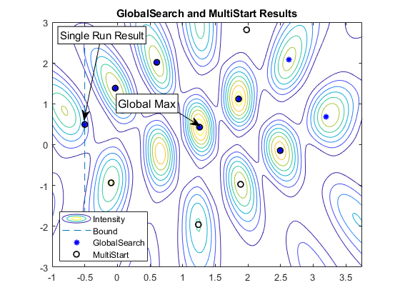
両方のソルバーが返した結果を調べてみましょう。注意すべき重要な点は、各ソルバーに対して作成されたランダムな開始ポイントに基づいて結果が異なることです。この例をもう一度実行すると、異なる結果になる可能性があります。最良の結果である xgs と xms の座標がコマンド ラインに出力されました。GlobalSearch と MultiStart によって返された固有の結果を示し、大域解への近さという観点から、各ソルバーの最良の結果を強調表示します。
各ソルバーの 5 番目の出力は、見つかった個別の最小値 (この場合は最大値) を含むベクトルです。結果の (x,y) ペアである solsgs と solsms を、前に使用した等高線プロットに対してプロットします。
% Plot GlobalSearch results using the '*' marker
xGS = cell2mat({solsgs(:).X}');
scatter(xGS(:,1),xGS(:,2),'*','MarkerEdgeColor',[0 0 1],'LineWidth',1.25)

% Plot MultiStart results using a circle marker
xMS = cell2mat({solsms(:).X}');
scatter(xMS(:,1),xMS(:,2),'o','MarkerEdgeColor',[0 0 0],'LineWidth',1.25)
legend('Intensity','Bound','GlobalSearch','MultiStart','Location','best')

title('GlobalSearch and MultiStart Results')
境界を緩める
問題の境界が厳しかったため、GlobalSearch と MultiStart の両方がこの実行でグローバル最大値を見つけることができました。
目的関数や制約についてあまり知られていない場合、厳密な境界を見つけることは実際には難しい場合があります。ただし、一般的には、開始点のセットを制限する適切な領域を推測することはできるかもしれません。説明のために、境界を緩和して、開始点を生成するより広い領域を定義し、ソルバーを再試行してみましょう。
% Relax the bounds to spread out the start points
problem.lb = -5*ones(2,1);
problem.ub = 5*ones(2,1);

% Run GlobalSearch
tic;
[xgs,~,~,~,solsgs] = run(gs,problem);
toc
xgs

% Run MultiStart with 15 randomly generated points
tic;
[xms,~,~,~,solsms] = run(ms,problem,15);
toc
xms
GlobalSearch stopped because it analyzed all the trial points.

All 4 local solver runs converged with a positive local solver exit flag.
Elapsed time is 0.173760 seconds.

xgs =

    0.6571   -0.2096


MultiStart completed the runs from all start points.

All 15 local solver runs converged with a positive local solver exit flag.
Elapsed time is 0.134150 seconds.

xms =

    2.4947   -0.1439
% Show the contours
figure
contour(X,Y,Z)
hold on

% Create textarrow showing the location of xglobal
annotation('textarrow',[0.44 0.50],[0.63 0.58],'TextEdgeColor',[0 0 0],...
    'TextBackgroundColor',[1 1 1],'FontSize',12,'String',{'Global Max'});
axis([-1 3.75 -3 3])

% Plot GlobalSearch results using the '*' marker
xGS = cell2mat({solsgs(:).X}');
scatter(xGS(:,1),xGS(:,2),'*','MarkerEdgeColor',[0 0 1],'LineWidth',1.25)

% Plot MultiStart results using a circle marker
xMS = cell2mat({solsms(:).X}');
scatter(xMS(:,1),xMS(:,2),'o','MarkerEdgeColor',[0 0 0],'LineWidth',1.25)

% Highlight the best results from each:
% GlobalSearch result in red, MultiStart result in blue
plot(xgs(1),xgs(2),'sb','MarkerSize',12,'MarkerFaceColor',[1 0 0])
plot(xms(1),xms(2),'sb','MarkerSize',12,'MarkerFaceColor',[0 0 1])
legend('Intensity','GlobalSearch','MultiStart','Best GS','Best MS','Location','best')

title('GlobalSearch and MultiStart Results with Relaxed Bounds')
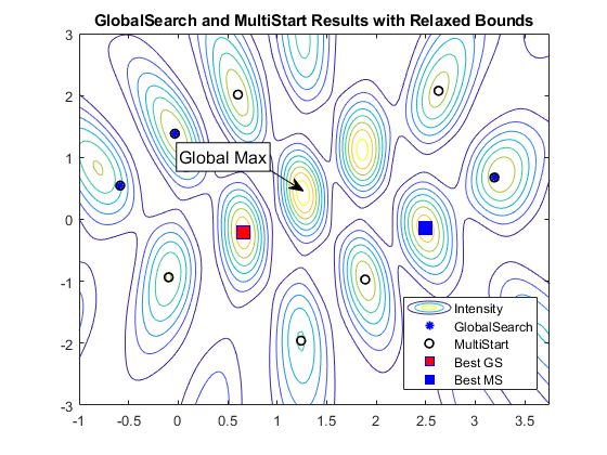
GlobalSearch からの最良の結果は赤い四角で示され、MultiStart からの最良の結果は青い四角で示されます。
GlobalSearchパラメーターの調整
この実行では、境界によって定義されたより広い領域が与えられたため、どちらのソルバーも最大強度のポイントを特定できなかったことに注意してください。これを克服するにはいくつかの方法があります。まず、GlobalSearch を調べます。
GlobalSearch は fmincon を数回しか実行していないことに注意してください。グローバル最大値を見つける可能性を高めるために、より多くのポイントを実行したいと思います。開始点セットをグローバル最大値を見つける可能性が最も高い候補に制限するには、StartPointsToRun プロパティを bounds-ineqs に設定して、制約を満たさない開始点を無視するように各ソルバーに指示します。さらに、GlobalSearch が狭いピークを素早く識別できるように、MaxWaitCycle および BasinRadiusFactor プロパティを設定します。MaxWaitCycle を減らすと、GlobalSearch により、デフォルト設定よりも頻繁に引き込み領域の半径が BasinRadiusFactor だけ減少します。
% Increase the total candidate points, but filter out the infeasible ones
gs = GlobalSearch(gs,'StartPointsToRun','bounds-ineqs', ...
    'MaxWaitCycle',3,'BasinRadiusFactor',0.3);
% Run GlobalSearch
tic;
xgs = run(gs,problem);
toc
xgs
GlobalSearch stopped because it analyzed all the trial points.

All 10 local solver runs converged with a positive local solver exit flag.
Elapsed time is 0.242955 seconds.

xgs =

    1.2592    0.4284
MultiStartの並列機能の活用
グローバル最大値を見つける可能性を高めるための強引な方法は、単純に開始点を増やすことです。繰り返しますが、これはすべての状況で実用的であるとは限りません。私たちの場合、これまでは小さなセットのみを試しており、実行時間もそれほど長くありませんでした。したがって、より多くの開始ポイントを試してみるのは合理的です。計算を高速化するために、Parallel Computing Toolbox ™ が利用可能な場合は MultiStart を並列に実行します。
% Set the UseParallel property of MultiStart
ms = MultiStart(ms,'UseParallel',true);

try
    demoOpenedPool = false;
    % Create a parallel pool if one does not already exist
    % (requires Parallel Computing Toolbox)
    if max(size(gcp)) == 0 % if no pool
        parpool
        demoOpenedPool = true;
    end
catch ME
    warning(message('globaloptim:globaloptimdemos:opticalInterferenceDemo:noPCT'));
end

% Run the solver
tic;
xms = run(ms,problem,100);
toc
xms

if demoOpenedPool
    % Make sure to delete the pool if one was created in this example
    delete(gcp) % delete the pool
end
MultiStart completed the runs from all start points.

All 100 local solver runs converged with a positive local solver exit flag.
Elapsed time is 0.956671 seconds.

xms =

    1.2592    0.4284
客観的制約と非線形制約
ここでは、最適化問題を定義する関数をリストします。
function p = waveIntensity(x,amp,phase,relFreqConst,numSources,origins)
% WaveIntensity Intensity function for opticalInterferenceDemo.

%   Copyright 2009 The MathWorks, Inc.

d = distanceFromSource(x,numSources,origins);
ampVec = [sum(amp./d .* cos(phase - d*relFreqConst));
    sum(amp./d .* sin(phase - d*relFreqConst))];

% Intensity is ||AmpVec||^2
p = ampVec'*ampVec;
function [c,ceq] = apertureConstraint(x,xcoords,ycoords)
% apertureConstraint Aperture constraint function for opticalInterferenceDemo.

%   Copyright 2009 The MathWorks, Inc.

ceq = [];
c = (x(1) - xcoords).^2 + (x(2) - ycoords).^2 - 9;
function d = distanceFromSource(v,numSources,origins)
% distanceFromSource Distance function for opticalInterferenceDemo.

%   Copyright 2009 The MathWorks, Inc.

d = zeros(numSources,1);
for k = 1:numSources
    d(k) = norm(origins(k,:) - [v 0]);
end