Field-Oriented Control of PMSM Using Fuzzy PI Controller

This example shows you how to use a fuzzy PI controller for speed control of a permanent magnet synchronous motor (PMSM) using field-oriented control (FOC) principles. It requires Motor Control Blockset™ and Global Optimization Toolbox software.

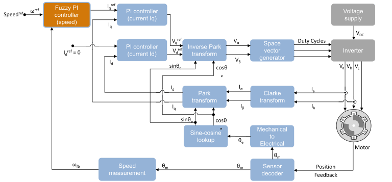
For more details about FOC, see Field-Oriented Control (FOC) (Motor Control Blockset). The following figure shows an FOC architecture, where a fuzzy PI controller regulates the q-axis current for speed control, whereas classical PI controllers regulate the d-axis and q-axis stator voltages to drive the motor at the required speed. The speed-tracking performance of an FOC algorithm using a fuzzy PI controller is similar to that of a classical PI-controller-based FOC.

PMSM Model

Open the mcb_pmsm_foc_fuzzy Simulink® model.

model = "mcb_pmsm_foc_fuzzy";
open_system(model);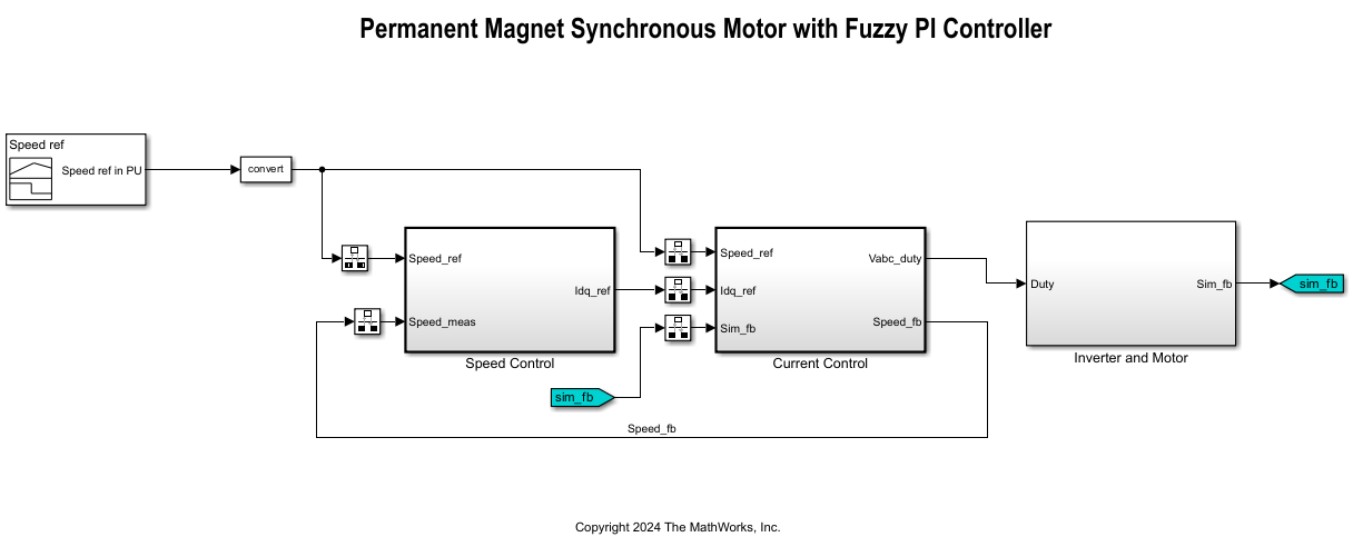

When you open the model, it loads the configured parameters including the motor parameters to the workspace for simulation. To view and update these parameters, open the mcb_pmsm_foc_params.m model initialization script file. For details about the control parameters and variables available in this script, see Estimate Control Gains and Use Utility Functions (Motor Control Blockset).

You can select and access the fuzzy PI controller inside the Speed Control subsystem by running this command.

SpeedController = "FL";
open_system(model + "/Speed Control/Speed Controller");

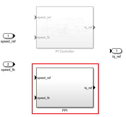
The fuzzy logic controller uses a proportional-integral (PI) configuration, where a fuzzy inference system (FIS) uses speed error and its derivative values to generate required q-axis current values to maintain the required speed of the motor.

open_system(model + "/Speed Control/Speed Controller/FPI");

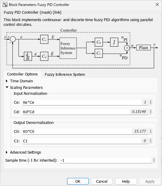
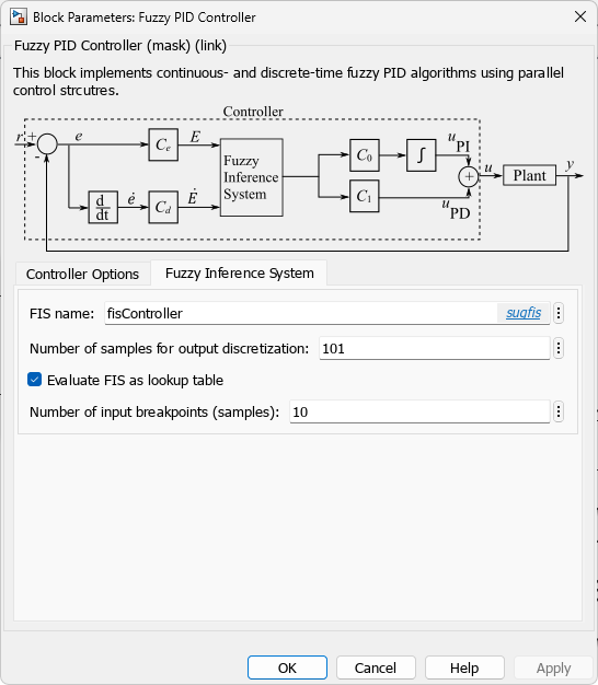
The model configuration parameters include the following parameters for Fuzzy PID Controller block.

Kp = PI_params.Kp_speed;
Ki = PI_params.Ki_speed;
Ce = 1;
C0 = Ki/Ce;
Cd = Ce*Kp/Ki;
C1 = 0;
Ke = 1;
Kd = 1;
K0 = 1;
fisController = readfis('fuzzycontroller');

Here:

• The values of the controller scaling factors, Ce, C0, and Cd are derived from the conventional PI controller gains.

• The Cd scaling factor is zero for a PI controller configuration.

• The multiplying factors Ke, Kd, and K0 are included for further tuning of the scaling parameter values.

• The default FIS, fuzzycontroller, is a linear FIS, which aids in computing the initial controller scaling factors.

• The FIS lookup table option is used for faster simulation of the fuzzy system.

The following figures show the Fuzzy Logic Controller block configuration.

Tune Scaling Parameters

The initial scaling parameter values of the fuzzy controller are calculated using the tuned gain values (Kp and Ki) of a PI controller.

You can, however, further tune the scaling parameter values for a better performance of the controller. This example tunes the multiplying factors Ke, Kd, and K0 of the scaling parameters Ce, Cd, and C0 respectively.

Set runtune flag to true to tune the scaling parameters using an optimization algorithm; otherwise, set runtune to false to load pre-tuned scaling parameter values.

runtune = false;

Create an options set for particle swarm optimization method. Specify ObjectiveLimit, InitialSwarmMatrix, MaxIterations, and Display option values for this optimization problem.

options = optimoptions("particleswarm", ...
        ObjectiveLimit=0, ...
        InitialSwarmMatrix=[1 1 1], ...
        MaxIterations=5, ...
        Display="none");

Use default random number generation seed to reproduce the tuning results.

rng("default")

Tune the scaling parameters of the fuzzy controller.

h = figure;
h.Position(4) = 500;
if runtune
    optimData = ParameterOptimizationData(); % Data storage for tuning results.
    ranges = [0.5 0.5 0.5;1 1 2.5]; % Parameter range values.
    particleSwarmSearch(model,ranges,optimData,options); % Tune parameter values.

    save fuzzyFOCExampleData optimData % Save tuning results.
else
    data = load("fuzzyFOCExampleData.mat"); % Load tuning results.
    optimData = data.optimData;
    labels = getTuningLabels();
    plotData(optimData,labels)
end

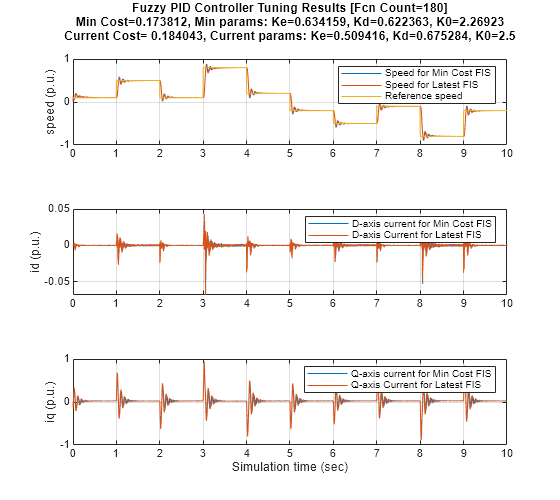
Ke = optimData.MinKe

Ke = 
0.6342

Kd = optimData.MinKd

Kd = 
0.6224

K0 = optimData.MinK0

K0 = 
2.2692

The multiplying factors are tuned to optimize the integral of absolute speed error.

Compare FIS with PI Controllers

Simulate the conventional PI controller and compare the performance with the fuzzy PI controller.

compareWithPIController(model,optimData)

The tuned fuzzy PI controller shows better speed tracking results (using integral of absolute speed error) as compared to the PI controller.

Next Steps

• You can further introduce nonlinearity to the fuzzy controller using nonlinear membership functions (MFs).

• You can tune the MFs parameter values for improved controller performance.

• You can also replace the PI controllers with fuzzy controllers for stator voltage regulation.

Local Functions

function compareWithPIController(model,fisControllerCost)
%% Simulate model with PI controller to compare with FIS controller. 

% Simulate model and get data.
assignin('base','SpeedController','PI')
out = sim(model);
costData = ParameterOptimizationData;
costData.RefSpeed = out.refSpeed.Data;
costData.Tout = out.refSpeed.Time;
costData.MinSpeed = fisControllerCost.MinSpeed;
costData.SimSpeed = out.simSpeed.Data;
costData.MinId = fisControllerCost.MinId;
costData.SimId = out.simId.Data;
costData.MinIq = fisControllerCost.MinIq;
costData.SimIq = out.simIq.Data;

% Calculate cost.
cost = out.speedIAE.Data(end);%sqrt(meanSquare);
costData.CurrCost = cost;
costData.MinCost = fisControllerCost.MinCost;

% Plot data
labels.plotTitleFormat = 'Fuzzy PI controller cost = %g, PI controller cost = %g\n';
labels.speedLegend = ["Speed for FIS Controller" "Speed for PI Controller" "Reference Speed"];
labels.idLegend = ["D-axis current for FIS Controller" "D-axis current for PI Controller"];
labels.iqLegend = ["Q-axis current for FIS Controller" "Q-axis current for PI Controller"];
labels.isTuningResults = false;

h = figure;
h.Position(4) = 500;
plotData(costData,labels)
end

function particleSwarmSearch(model,ranges,costData,options)
%% Use particle swarm method to find a solution.

% Reset cost data.
reset(costData)

% Create an optimization problem using particle swarm.
p = struct(...
    'solver','particleswarm', ...
    'objective',@(x)fpiOptimCostFcn(x,model,costData), ...
    'nvars',size(ranges,2), ...
    'lb',ranges(1,:), ...
    'ub',ranges(2,:), ...
    'options',options, ...
    'rngstate',[]  ...
    );

% Find a cost-optimized solution.
particleswarm(p);
end