Test Generated Code with PIL Simulations on Renesas RA Microcontrollers
This example shows how to use the Embedded Coder ® Support Package for Renesas® RA Microcontrollers to generate code from Simulink models and perform Processor-in-the-Loop (PIL) simulations on the Renesas RA6T2 board. You can run this workflow using either the SIL/PIL Manager or command-line approach. PIL verification is a key step in validating that the generated code, when executed on actual hardware, replicates the behavior of your original Simulink design. For more information, see Choose a SIL or PIL Approach and SIL/PIL Manager.
During a PIL simulation, your algorithm runs directly on the Renesas hardware while the host computer manages simulation scheduling, generates input signals, and communicates with the controller via a serial interface. This configuration allows you to verify numerical equivalence between simulation and hardware execution, measure algorithm execution time, and analyze memory usage on the target device.
Prerequisites
Complete the Hardware Setup for Embedded Coder Support Package for Renesas RA Microcontrollers.
Go through SIL/PIL Manager documentation.
Required Hardware
Renesas RA6T2 based board (RA6T2 MCK)
USB type C cable
FTDI Friend (This example was tested using FTDI Friend USB TTL-232R 3.3V adapter
Hardware Connection
When using an FTDI adapter for communication between the host computer and the Renesas RA6T2 target board, make the following connections.
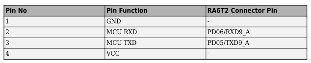
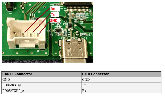
The Rx, Tx, and GND labels shown in red in the figure indicate the corresponding pins on the FTDI connector.
Configure the Simulink Model
Open the
PILCounter.slxSimulink model.
modelName = "PILCounter.slx";
open_system(modelName)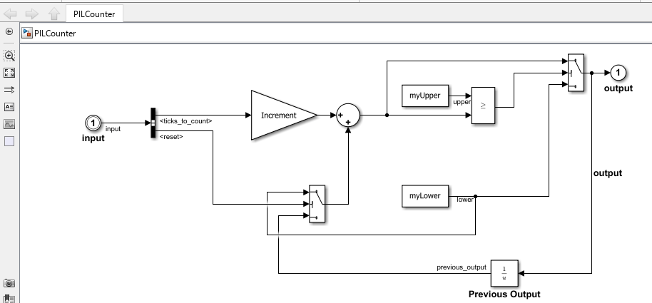
2. In the Simulink model, click Modeling > Model Settings to open the Configuration Parameters dialog box.
3. In the Configuration Parameters dialog box, navigate to Hardware Implementation > Hardware board and select Renesas RA6 Based board.
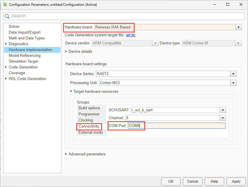
4. Navigate to Target hardware resources > Connectivity and enter the COM Port number. To find the COM port number, check the Device Manager on your PC.
Note: Ensure you provide a valid COM port. Using an invalid port may trigger a confusing error message, possibly including an error ID.
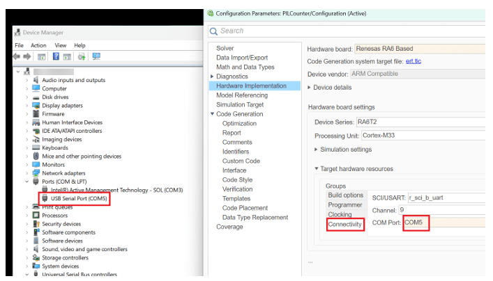
These instructions assume that UART Channel 9 is being used, with the default instance name (g_uart9) as specified in the standard configuration.xml file.
5. Click Apply and OK.
Verify Referenced Model Code Using PIL (SIL/PIL Manager Workflow)
The SIL/PIL Manager simplifies the process of simulating and verifying of generated code on your target with a single click. This example shows how to verify the generated code for a referenced model by running a PIL simulation.
With this approach:
You can verify code generated for referenced models.
You must provide a test harness model to supply test vectors or stimulus inputs.
You can easily switch a Model block between normal and PIL simulation mode.
To verify the reference model, perform these steps:
1. Open the PILModelBlock.slx model. This model contains referenced model block and stimulus inputs. You will configure the Model block to run in PIL mode.
modelName = 'PILModelBlock.slx';
open_system(modelName)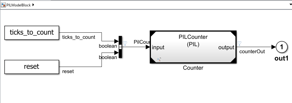
2. Configure and run the Counter Model block in PIL mode.
Right click the CounterA block and select
Processor-in-the-loop (PIL)for Simulation Mode option andModel Referencefor Code Interface option.
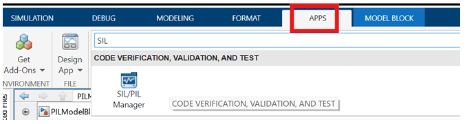
3. In the Simulink toolstrip, click Apps and then select SIL/PIL Manager.
4. Select Model blocks in SIL/PIL mode in the System Under Test option.
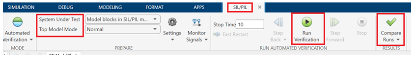
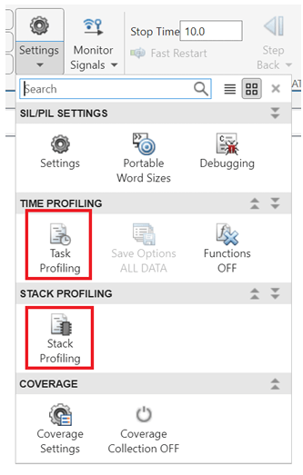
5. Select the appropriate options in the settings to view execution-time metrics or stack profiling in addition to numerical equivalence. Note that Task profiling and Stack profiling are mutually exclusive, select only one profiling mode at a time. Selecting both options together can result in an error during SIL/PIL setup or execution.
For more information, see Choose a SIL or PIL Approach and SIL/PIL Manager. In this example, only numerical equivalence is tested. Coverage settings appear only if you have a license for Simulink Coverage.
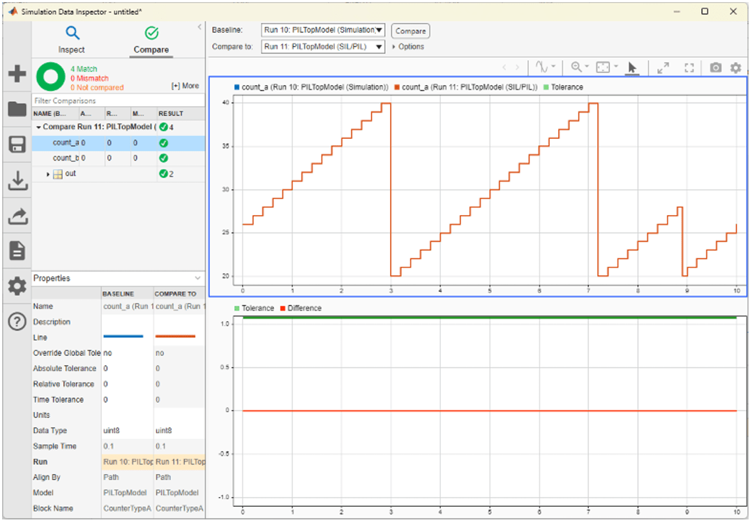
6. Click Run Verification to start the simulation. Compare Runs displays the numerical equivalence between PIL simulation output and the normal mode simulation output.
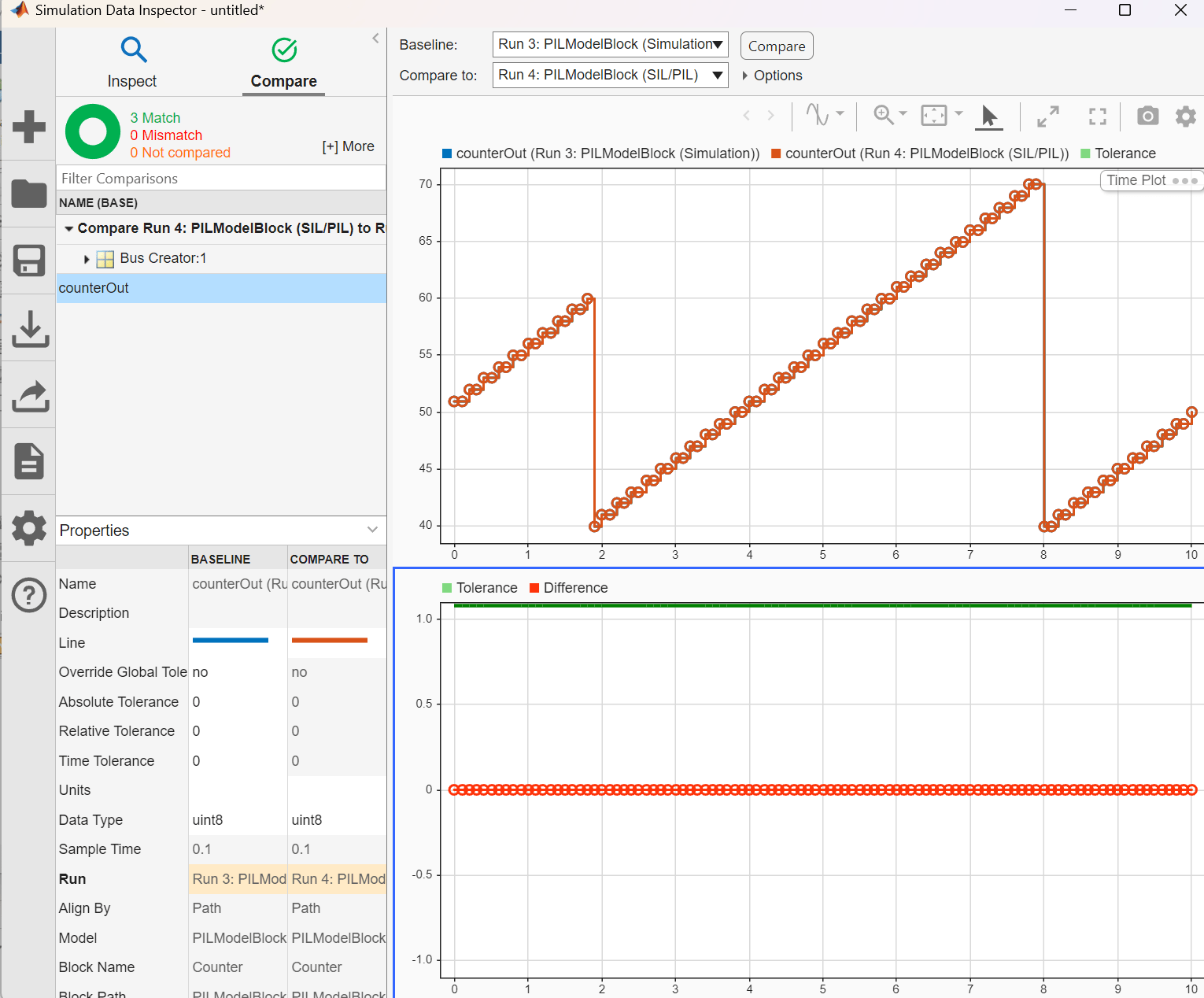
Observe that the reset signal forces the output to return to its lower limit of 40 at the 19th sample. Additionally, the difference signal highlights the numerical equivalence between the host simulation and the PIL simulation, allowing you to verify that both executions produce consistent results.
Verify Top Model Code Using PIL (SIL/PIL Manager Workflow)
This section shows how to verify the generated code for a top-level model by running a Processor-in-the-Loop (PIL) simulation using the SIL/PIL Manager.
With this approach:
You can verify code generated for top model.
You must configure the model to load test vectors or stimulus inputs from the MATLAB workspace.
You can easily switch the entire model between normal and PIL simulation mode.
To verify the model, perform these steps:
1. Open the PILTopModel.slx model. This model is configured for the Renesas RA6 Based target and perform the steps mentioned in 'Hardware Connections and Simulink Model Configuration' section.
modelName = "PILTopModel.slx";
open_system(modelName)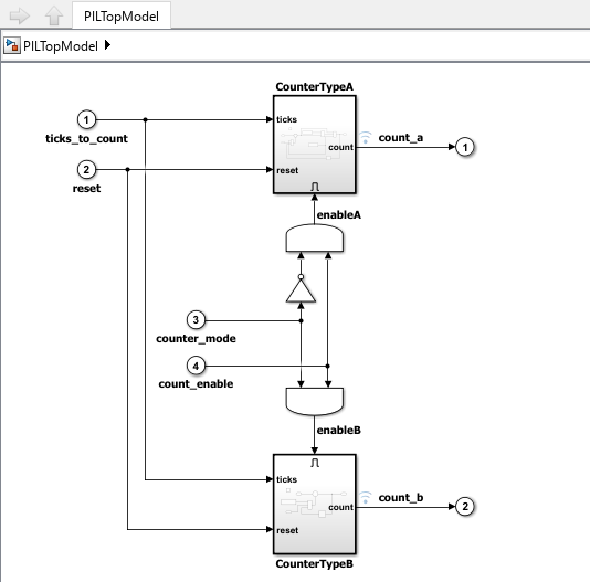
2. In the Simulink toolstrip, click Apps and then select SIL/PIL Manager.
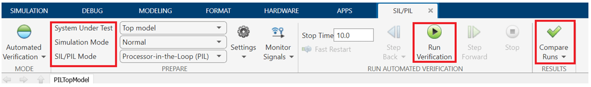
3. For System Under Test option, select Top model and for Simulation Mode option, select Normal or Accelerator.
4. Click Run Verification to start the simulation. Compare option displays the numerical equivalence between PIL simulation output and the normal mode simulation output.
PIL Simulation of a Model Block Using the Command Line
This section shows how to implement the previously discussed workflow using a command-line approach. You will test the generated model code by running a test harness model that executes a Model block in PIL mode.
With this approach:
You can test code generated from either a top model or a referenced model. The code from the top model uses the standalone code interface, while the code from the referenced model uses the model reference code interface. For more information, see Code Interfaces for SIL and PIL.
You use a test harness model or a system model to provide test vector or stimulus inputs.
You can easily switch a Model block between the normal and PIL simulation modes.
Perform these steps:
1. Open the PILModelBlock.slx model.
model = "PILModelBlock";
open_system(model)
2. Perform the steps listed in Configure the Simulink Model section to select the hardware board and COM port.
3. Turn off the following options:
Code coverage
Execution time profiling
coverageSettings = get_param(model, 'CodeCoverageSettings');
coverageSettings.CoverageTool='None';
set_param(model, 'CodeCoverageSettings',coverageSettings);
open_system(model)
set_param(model, 'CodeExecutionProfiling','off');
open_system('PILCounter')
set_param('PILCounter', 'CodeExecutionProfiling','off');
currentFolder=pwd;
save_system('PILCounter', fullfile(currentFolder,'PILCounter.slx'))
4. Configure state logging for the models.
set_param('PILCounter', 'SaveFormat','Dataset');
save_system('PILCounter', fullfile(currentFolder,'PILCounter.slx'))
set_param(model, 'SaveFormat','Dataset');
set_param(model, 'SaveState','on');
set_param(model, 'StateSaveName', 'xout');
Test Top Model Code
For the Model block in PIL mode, specify generation of top-model code, which uses the standalone code interface.
set_param([model '/Counter'],"SimulationMode",'Processor-in-the-loop (PIL)');
set_param([model '/Counter'], 'CodeInterface', 'Top model');
Run a simulation of the test harness model.
out = sim(model,10);
The Model block running in PIL mode operates as a separate process on your computer. In the working folder, model reference code is generated unless code from a previous build already exists.
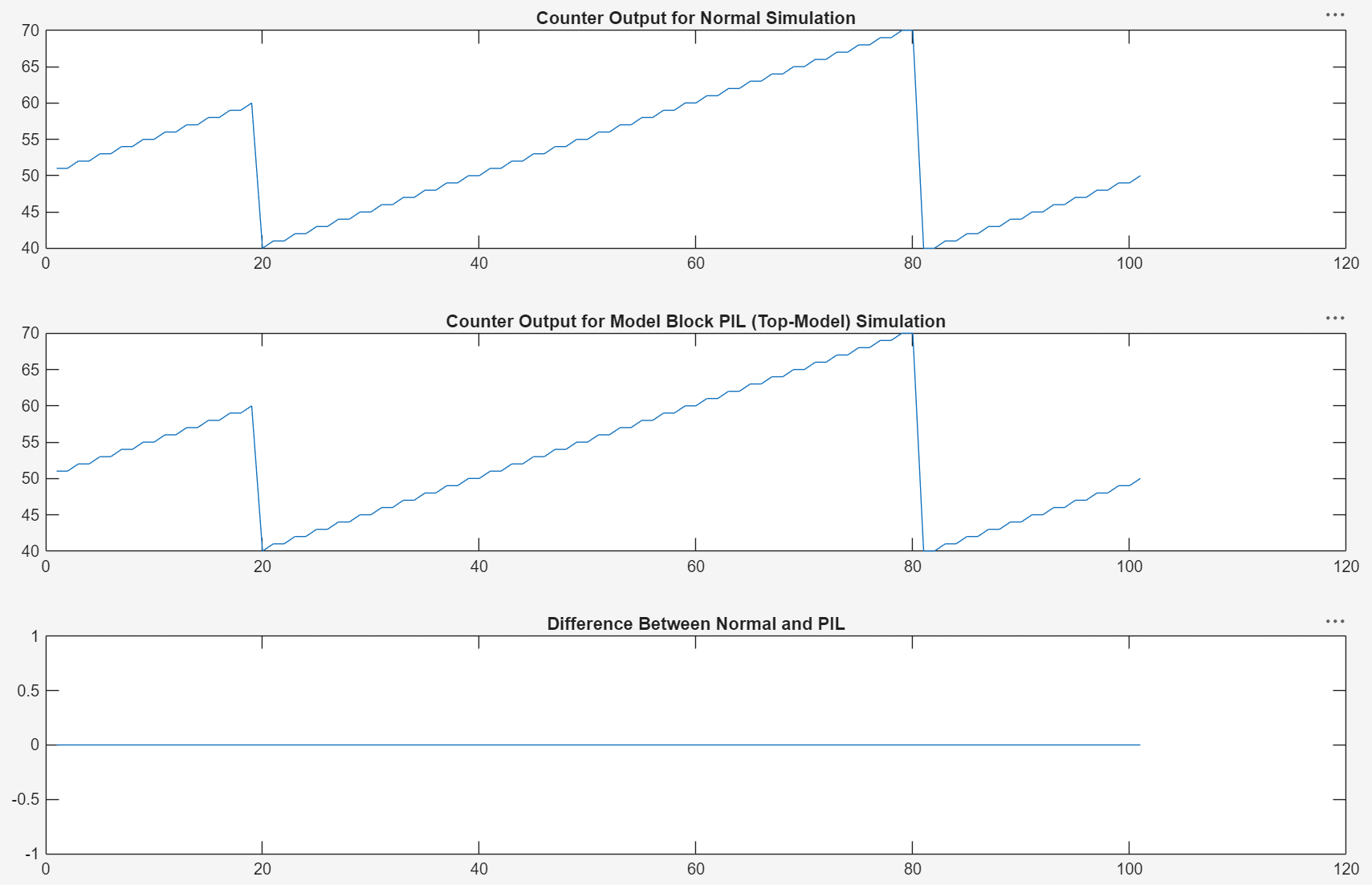
Compare the behavior of Model block in normal and PIL mode.
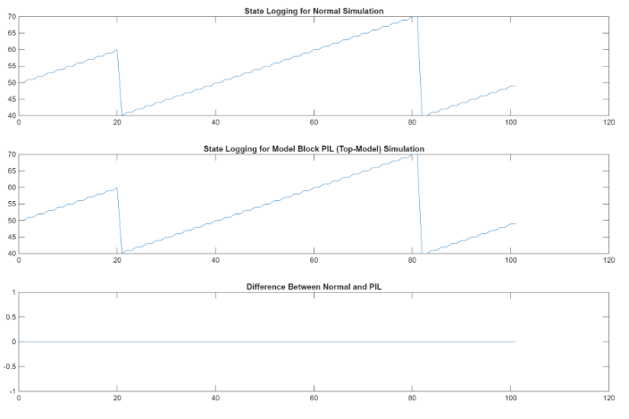
PIL mode:
yout = out.logsOut;
yout_pil = yout.get('counterOut').Values.Data;
xout2 = out.xout;
xout2_pil = xout2{1}.Values.Data;

Normal mode:
set_param([model '/Counter'],"SimulationMode","Normal")
out = sim(model,10);

yout = out.logsOut;
yout_normal = yout.get('counterOut').Values.Data;
xout2 = out.xout;
xout2_normal = xout2{1}.Values.Data;

fig1 = figure;
subplot(3,1,1), plot(yout_normal), title('Counter Output for Normal Simulation')
subplot(3,1,2), plot(yout_pil), title('Counter Output for Model Block PIL (Top-Model) Simulation')
subplot(3,1,3), plot(yout_normal-yout_pil), ...
    title('Difference Between Normal and PIL');

fig2 = figure;
subplot(3,1,1), plot(xout_pil), title('State Logging for Normal Simulation')
subplot(3,1,2), ...
    plot(xout_normal), title('State Logging for Model Block PIL (Top-Model) Simulation')
subplot(3,1,3), plot(xout_normal-xout_pil), ...
    title('Difference Between Normal and PIL');
Clean up.
close_system(model,0);
close_system('PILCounter',0);
if ishandle(fig1), close(fig1), end, clear fig1
if ishandle(fig2), close(fig2), end, clear fig2
if ishandle(fig3), close(fig3), end, clear fig3
if ishandle(fig4), close(fig4), end, clear fig4
simResults={'out','yout','yout_pil','yout_normal', ...
    'out2','yout2','yout2_pil','yout2_normal', ...
    'PilCounterBus','T','reset','ticks_to_count','Increment'};
save([model '_results'],simResults{:});
clear(simResults{:},'simResults')
Test Model Reference Code
For the Model block in PIL mode, specify generation of referenced model code, which uses the model reference code interface.
set_param([model '/Counter'],"SimulationMode",'Processor-in-the-loop (PIL)');
set_param([model '/Counter'], 'CodeInterface', 'Model reference');
Run a simulation of the test harness model.
out2 = sim(model,20);
The model block in PIL mode runs as a separate process on your computer. In the working folder, you see that model reference code is generated unless code from a previous build exists.
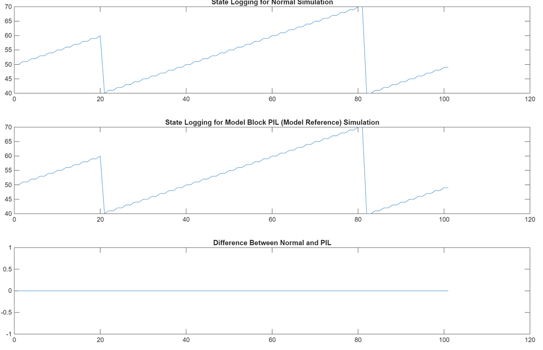
Compare the behavior of Model blocks in normal and SIL modes. The results match.
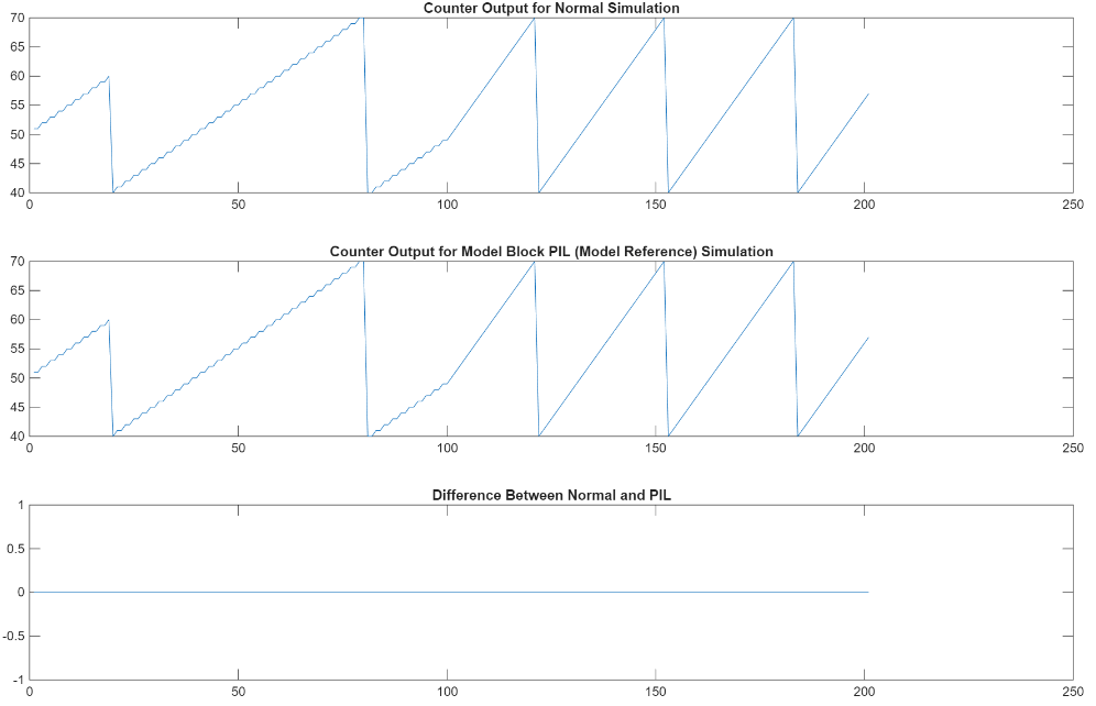
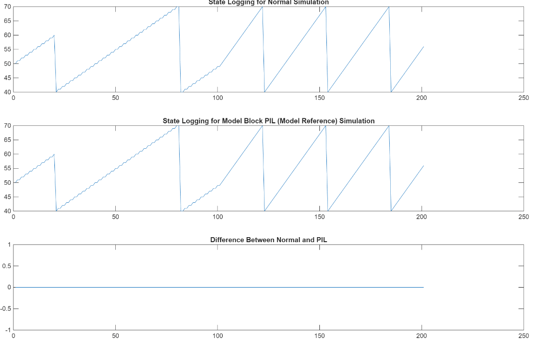
PIL mode:

yout2 = out2.logsOut;
yout2_pil = yout2.get('counterOut').Values.Data;
xout2 = out2.xout;
xout2_pil = xout2{1}.Values.Data;


Normal Mode:
set_param([model '/Counter'],"SimulationMode","Normal");
out2 = sim(model,20);

yout2 = out2.logsOut;
yout2_normal = yout2.get('counterOut').Values.Data;
xout2 = out2.xout;
xout2_normal = xout2{1}.Values.Data;


fig3 = figure;
subplot(3,1,1), plot(yout2_normal), title('Counter Output for Normal Simulation')
subplot(3,1,2), ...
    plot(yout2_pil), title('Counter Output for Model Block PIL (Model Reference) Simulation')
subplot(3,1,3), plot(yout2_normal-yout2_pil), ...
    title('Difference Between Normal and PIL');


fig4 = figure;
subplot(3,1,1), plot(xout2_pil), title('State Logging for Normal Simulation')
subplot(3,1,2), ...
    plot(xout2_normal), title('State Logging for Model Block PIL (Model Reference) Simulation')
subplot(3,1,3), plot(xout2_normal-xout2_pil), ...
    title('Difference Between Normal and PIL');
PIL Simulation for a Top-Level Model Using the Command Line
Test generated model code by running a top-model PIL simulation. With this approach:
You test code generated from the top model, which uses the standalone code interface.
You configure the model to load test vectors or stimulus inputs from the MATLAB workspace.
You can easily switch the top model between the normal and PIL simulation modes
Perform these steps:
1. Open a simple counter top model.
model = "PILTopModel";
open_system(model)
2. Update the required settings in the configset.
cs = getActiveConfigSet(model);
cs.set_param('HardwareBoard','Renesas RA6 Based');
cs.openDialog;
3. Perform the steps listed in Configure the Simulink Model section to select the hardware board and COM port.
4. To focus on numerical equivalence testing, turn off the following options:
Model coverage
Code coverage
Execution time profiling
set_param(gcs, 'RecordCoverage','off');
coverageSettings = get_param(model, 'CodeCoverageSettings');
coverageSettings.CoverageTool='None';
set_param(model, 'CodeCoverageSettings',coverageSettings);
set_param(model, 'CodeExecutionProfiling','off');
5. Configure the input stimulus data.
set_param(model, 'LoadExternalInput','on');
set_param(model, 'ExternalInput','ticks_to_count, reset, counter_mode, count_enable');
set_param(model, 'SignalLogging', 'on');
set_param(model, 'SignalLoggingName', 'logsOut');
set_param(model, 'SaveOutput','on')
6. Run a normal mode simulation.
set_param(model,'SimulationMode','normal')
sim_output = sim(model,10);
yout_normal = [sim_output.yout.signals(1).values sim_output.yout.signals(2).values];
7. Run a top-model PIL simulation. Delete slprj folder that might have be created in previous runs.
set_param(model,'SimulationMode','Processor-in-the-Loop (PIL)')
sim_output = sim(model,10);
yout_pil = [sim_output.yout.signals(1).values sim_output.yout.signals(2).values];
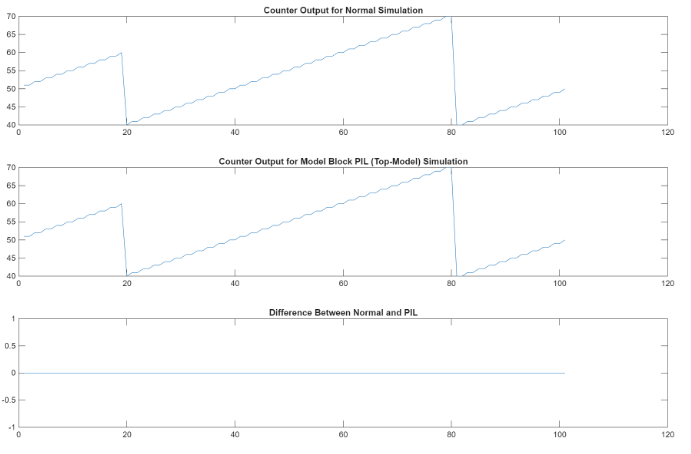
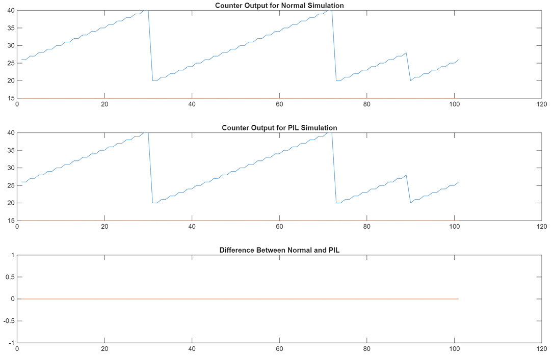
If up-to-date code for this model does not exist, Simulink generates and compiles new code. The generated code runs as a separate process on your computer. Plot and compare the results of the normal and PIL simulations, and observe that the results match.
fig1 = figure;
subplot(3,1,1), plot(yout_normal), title('Counter Output for Normal Simulation')
subplot(3,1,2), plot(yout_pil), title('Counter Output for PIL Simulation')
8. Clean up.
close_system(model,0);
if ishandle(fig1), close(fig1), end
clear fig1
simResults = {'yout_pil','yout_normal','model','T',...
    'ticks_to_count','reset'};
save([model '_results'],simResults{:});
clear(simResults{:},'simResults')