Choose Data Types for Biquad Filter
This example shows how to choose fixed-point data types for biquad filter implementation on hardware.
Choosing quantization settings for biquad filters can be challenging. Unlike feed-forward filters such as FIR filters, biquad filters are feed-back, or recursive, filters and have denominators that make fixed-point analysis more difficult.
The key step to choosing data types for any kind of fixed-point filter is to find the maximum output value.
Finite Impulse Response Filters
For an FIR filter, the maximum output value is the largest input value applied repeatedly, multiplied by the coefficients, and summed. An important detail is that for a negative coefficient, the largest input value must be a negative value. The coefficients of an FIR filter are also the impulse response of the filter, so you can find the maximum output value by summing the absolute value of the impulse response and multiplying that by the largest input value. The sum of the absolute value of a vector is also called the 1-norm, equivalent to calling norm(x,1).
Infinite Impulse Response Filters
Since biquad filters are infinite impulse response filters, their impulse response can theoretically go on forever. In practice, you consider the impulse response only until the result falls below an arbitrary threshold. The impulse response calculations in this example use a threshold of 1e-5, but it could be any value that makes sense for your system.
This analysis also assumes that you have a bounded-input, bounded-output (BIBO) filter. This condition is generally true unless you are building an oscillator rather than a filter. Another way of stating that the filter is BIBO is the 1-norm of the impulse response exists. Yet another way to state BIBO stability is that all the poles of the filter are strictly inside the unit circle. Quantizing the filter coefficients can occasionally move the poles outside the unit circle, which would make the filter unstable, but this situation is rare.
You can think of the maximum output value as the maximum dynamic range, or gain, of the filter. For a maximum input value, you can compute the resulting output maximum value by multiplying by the 1-norm as shown above. If you consider ceil(log2(maxOutput)), you can think of the gain as the bit growth of the filter in the integer part of the output. The maximum value changes the dynamic range but not necessarily the precision.
Multi-Section IIR Filters
A further complication of biquad filters is that they can have multiple second-order sections with gain stages, called scale values, between the sections. Certain filter design methods, such as elliptic filters, have both very large and very small scale values, which results in large changes in dynamic range and is challenging for fixed-point settings. You can analyze the maximum value of each filter section individually, with and without the scale value gain.
Quantization Settings
In biquad filters, saturation or wrapping of values in the denominator changes the integrating part of the filter and affects all future calculations. The best practice is to choose fixed-point types that avoid overflows in the filter. It is important to understand how the quantization settings in the DSP HDL Toolbox™ biquad filter work in the different filter structures.
Direct form II: In the DF2 structure, there are two quantization points per section. The filter quantizes to the accumulator data type after the adder for the feedback (denominator) part of the filter. This setting also sets the data type for the state registers. The filter quantizes to the output data type at the output of each section. If your filter design has large dynamic range, set the output type to allow for the largest dynamic range. If you require a smaller final output range, you can add an external quantization step after the filter.
Direct form II transposed: In the DF2T structure, there are also two quantization settings, but they are different from DF2. The filter quantizes to the accumulator data type after the adders and the state registers for each section. The filter quantizes to the output data type at the final adder before the output. This data type also applies to the feedback (denominator). Again, if your filter design has large dynamic range, set the output type to accommodate the largest dynamic range.
Direct form I fully serial: In the DF1 serial structure, the filter quantizes to the accumulator data type before the adder. This setting also sets the data type for the states and intermediate section output values. In this structure the filter quantizes to the output data type at the final output. In the serial filter, all of the numerator, denominator, and scale value coefficients must have the same data type because they are stored in the same ROM. To determine the fraction length that works for all of the coefficients, combine them into one vector and call fi(vector,1,16) to see what fraction size fits them all. The DSP HDL Toolbox biquad filter uses this method to determine the fraction length when you specify only a word length.
Design a Filter
To explore the quantization options for a biquad filter, create a low-pass filter. This example shows an elliptical filter, which has large dynamic range. To make analysis easier, configure the design function to return a System object™.
N     = 6;    % Order
Fpass = 0.4;  % Passband Frequency
Apass = 3;    % Passband Ripple (dB)
Astop = 80;   % Stopband Attenuation (dB)
h  = fdesign.lowpass('N,Fp,Ap,Ast',N,Fpass,Apass,Astop);
Hd = design(h,'ellip',Systemobject=true);
Analyze the Filter Dynamic Range
Calculate the overall dynamic range increase by finding the 1-norm of the impulse response.
monolithicMaxOutput = norm(impz(Hd),1)
monolithicMaxOutput =

    2.4455
The norm seems well-behaved with a maximum output of 2.44 for 1.0 input, or bit growth of 2 bits. Now consider the individual sections, without the scale values for now.
for ii =1:3
  unscaledSectionMax(ii) = norm(impz(Hd.Numerator(ii,:),Hd.Denominator(ii,:)),1)
end
unscaledSectionMax =

   15.8895


unscaledSectionMax =

   15.8895   30.8974


unscaledSectionMax =

   15.8895   30.8974   25.6815
The results show maximum outputs of around 16, 31, and 26 for the three sections. So there is a large dynamic range increase even before considering the scale values.
The filter applies the scale values before each section. The final scale value is 1.0 and does not contribute any bit growth. This code calls impz with a cell array to represent a cascaded transfer function.
for ii =1:3
  scaledSectionMax(ii) = norm(impz({Hd.Numerator(ii,:),Hd.Denominator(ii,:),Hd.ScaleValues(ii)},"ctf"),1)
end
scaledSectionMax =

    9.3512


scaledSectionMax =

    9.3512   52.7922


scaledSectionMax =

    9.3512   52.7922    0.1403
With the scale factors included, the first section is scaled down from 16 to around 9, but the second section is scaled up from 31 to 53, and the third section is scaled way down from 26 to about 0.14 due to the third scale value being 0.005. These scaled values give a clearer picture of the gain in this three-section filter.
Calculate Bit Growth
Compute the bit growth at each section, including the scale values.
for ii =1:3
  sectionBitGrowth(ii) = ceil(log2(norm(impz({Hd.Numerator(ii,:),Hd.Denominator(ii,:),Hd.ScaleValues(ii)},"ctf"),1)))
end
sectionBitGrowth =

     4


sectionBitGrowth =

     4     6


sectionBitGrowth =

     4     6    -2
This calculation shows that the first filter section adds 4 bits to dynamic range, the second adds 6 bits, and the third takes away 2 bits. Next, compare that bit growth with the calculated growth considering the entire filter as a single part.
monolithicBitGrowth = ceil(log2(norm(impz(Hd),1)))
monolithicBitGrowth =

     2
The overall transfer function shows a growth of 2 bits but that result ignores the larger dynamic range in the second filter section. The scale value before the third section has a a reduction in dynamic range of 7 bits. Overall the transfer function of the filter has bit growth of about 8.8 bits, and the scale values have bit growth of -7.5 leading to the overall growth of about 1.3 bits. These numbers show why you must consider the filter sections and their scale values individually to understand the bit growth for this filter.
This filter also shows why the order of sections and scale values can have such a big effect on dynamic range in certain classes of filters.
There are many potential quantization points in biquad filters and the DSP HDL Toolbox biquad filter tries to minimize the number of settings while still allowing for good control. In particular, the filter uses the output data type not just for the primary output but also for the output of each filter section. This implementation works well when the dynamic range of the sections are similar, but in cases like this filter where there is a large difference in the dynamic range of the sections, you must select an output data type that accommodates possible quantization effects at each section.
Configure Filter Data Types
Now that you know that you need bit growth of 6 bits to accommodate the dynamic range of the second filter section, you can configure the data types for the biquad filter. This code shows one filter with the correct dynamic range growth of 6 bits, and another filter with the overall dynamic range of 2 bits to see the difference. The filters set rounding mode to Nearest and enable saturation in case of overflows.
Your system has a 10-bit input with 9 fractional bits. You choose 16 bits for the coefficients, which require 14 fractional bits. Normally, a 10-bit input and 16-bit coefficient would result in a 26-bit multiplier and some extra bits for the accumulator. From the analysis above, you know that this filter requires 6 extra bits to accommodate the dynamic range of the three-section filter. The accumulator size becomes 32 bits with 23 fractional bits for the full dynamic range filter. For the quantizing filter, you use 3 extra bits, which results in a 29-bit accumulator with 23 fractional bits. Both filters have the same output data type.
H2bit = dsphdl.BiquadFilter(Numerator=Hd.Numerator, ...
                           Denominator=Hd.Denominator, ...
                           ScaleValues=Hd.ScaleValues, ...
                           Structure="Direct form I fully serial", ...
                           CoefficientsDataType="Custom", ...
                           CustomCoefficientsDataType=numerictype(1,16,14), ...
                           RoundingMethod="Nearest", ...
                           OverflowAction="Saturate", ...
                           AccumulatorDataType="Custom", ...
                           CustomAccumulatorDataType=numerictype(1,29,23), ...
                           OutputDataType="Full precision");

H6bit = dsphdl.BiquadFilter(Numerator=Hd.Numerator, ...
                            Denominator=Hd.Denominator, ...
                            ScaleValues=Hd.ScaleValues, ...
                            Structure="Direct form I fully serial", ...
                            CoefficientsDataType="Custom", ...
                            CustomCoefficientsDataType=numerictype(1,16,14), ...
                            RoundingMethod="Nearest", ...
                            OverflowAction="Saturate", ...
                            AccumulatorDataType="Custom", ...
                            CustomAccumulatorDataType=numerictype(1,32,23), ...
                            OutputDataType="Full precision");
Simulate the Filter
Generate a test input signal of a 1000-sample swept sine wave of increasing frequency, using signed 10-bit values with 9 fractional bits.
signalIn = fi(chirp(0:499,0,999,0.124).',1,10,9);
Simulate the double-precision filter for reference using double-precision input.
Yd = Hd(double(signalIn)).';
Simulate the two filters. Since the serial biquad filter cannot accept a new sample every clock cycle, this code checks the valid and ready outputs and sends new inputs when the object can accept them.
[bOut,bvOut,brOut] = H2bit(signalIn(1),true);
[gOut,gvOut,grOut] = H6bit(signalIn(1),true);
ii = 2;
while ii <= 500
    if brOut
        [bOut(end+1),bvOut(end+1),brOut] = H2bit(signalIn(ii),true);
        [gOut(end+1),gvOut(end+1),grOut] = H6bit(signalIn(ii),true);
        ii = ii + 1;
    else
        [bOut(end+1),bvOut(end+1),brOut] = H2bit(signalIn(ii),false);
        [gOut(end+1),gvOut(end+1),grOut] = H6bit(signalIn(ii),false);
    end
end
for tt=1:75                             % collect remaining outputs
    [bOut(end+1),bvOut(end+1),brOut] = H2bit(cast(0,'like',signalIn),false);
    [gOut(end+1),gvOut(end+1),grOut] = H6bit(cast(0,'like',signalIn),false);
end
bvalidOut = bOut(bvOut); % select only the valid outputs
gvalidOut = gOut(gvOut);
Calculate the mean-squared error using the double-precision baseline computed above. Plot the expected output and the results of the two filters.
bmse = mean((double(bvalidOut)-Yd).^2)
gmse = mean((double(gvalidOut)-Yd).^2)

f=figure;
tiledlayout(4,1)
ax1=nexttile;
stem(signalIn)
legend(ax1,'signalIn')
ax2=nexttile;
stem(Yd)
legend(ax2,'Expected filter output')
ax3=nexttile;
stem(gvalidOut);
legend(ax3,'H6bit output (no overflow)')
ax4=nexttile;
stem(bvalidOut);
legend(ax4,'H2bit output (with overflows)')
bmse =

    0.1849


gmse =

   1.0360e-05
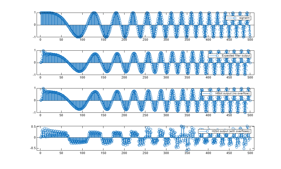
Now that you know how to choose data types that preserve the dynamic range in each section of a biquad filter and for the final output, you can explore further by changing from saturate to wrap overflow behavior. With appropriate fixed-point settings, the filter is not affected, but an over-quantized filter can have dramatic output swings. Since wrap behavior is significantly cheaper in hardware than saturate behavior, knowing how to set the quantization settings on biquad filters can save resources even with longer word lengths. The real benefit is avoiding any overflow of the denominator that would cause the filter to produce incorrect results.
See Also
Biquad Filter | dsphdl.BiquadFilter