勾配分布のプロットによる深層ニューラルネットワークの勾配消失の検出

この例では、深層ニューラルネットワークの学習中に勾配消失を監視する方法を説明します。

深いネットワークの学習では、"勾配消失" の問題がよく発生します。深層学習の学習アルゴリズムは、学習中にネットワークの学習可能なパラメーターを調整して損失を最小にすることを目的としています。勾配ベースの学習アルゴリズムは、現在の学習可能なパラメーターについての損失関数の勾配を使用して調整レベルを決定します。初期の層では、前の層から伝播された勾配を使用して勾配を計算します。そのため、常に 1 未満の勾配値を生成する活性化関数がネットワークに含まれている場合、更新アルゴリズムが初期の層に移動するにつれて、勾配の値が次第に小さくなります。その結果、ネットワークの初期の層はほとんど 0 に近い小さな勾配を受け取ることになり、ネットワークは学習ができなくなってしまいます。しかし、活性化関数の勾配が常に 1 以上であれば、勾配がネットワーク内をくまなく伝播でき、勾配消失が発生する可能性を減らすことができます。

この例では、異なる活性化関数をもつ 2 つのネットワークの学習を行い、勾配分布を比較します。

活性化関数の比較

活性化関数の特性の違いを説明するため、一般的な 2 つの深層学習活性化関数である ReLU およびシグモイドを比較します。

$ReLU (x) = {\begin{cases} x & x \geq 0 \\ 0 & x < 0 \end{cases}$

$Sigmoid (x) = {(1 + \exp (- x))}^{- 1}$

ReLU 活性化関数とシグモイド活性化関数の勾配を評価します。

x = linspace(-5,5,1000);

reluActivation = max(0,x);
reluGradient = gradient(reluActivation,0.01);

sigmoidActivation = 1./(1 + exp(-x));
sigmoidGradient = gradient(sigmoidActivation,0.01);

ReLU 活性化関数とシグモイド活性化関数、ならびにそれらの勾配をプロットします。

figure
tiledlayout(1,2)

nexttile
plot(x,[reluActivation;reluGradient])
legend("ReLU","Gradient of ReLU")

nexttile
plot(x,[sigmoidActivation;sigmoidGradient])
legend("Sigmoid","Gradient of Sigmoid")

ReLU の勾配は、全範囲で 0 または 1 です。そのため、ネットワーク内で勾配が逆伝播しても勾配が次第に小さくなることはなく、勾配消失が発生する可能性は減ります。シグモイドの勾配曲線は、全範囲で 1 未満です。そのため、シグモイド活性化層を含むネットワークは、勾配消失問題の影響を受ける可能性があります。

データの読み込み

digitTrain4DArrayData を使用して、5000 個の手書き数字の合成イメージとそのラベルから成る標本データを読み込みます。

[XTrain,TTrain] = digitTrain4DArrayData;
numObservations = length(TTrain);

学習イメージのサイズを自動的に変更するには、拡張イメージデータストアを使用します。

inputSize = [28,28,1];
augimdsTrain = augmentedImageDatastore(inputSize(1:2),XTrain,TTrain);

学習データ内のクラスの数を決定します。

classes = categories(TTrain);
numClasses = numel(classes);

ネットワークの定義

活性化層の効果を比較するため、2 つのネットワークを構築します。各ネットワークには、4 つの全結合層を隔てる ReLU 活性化層またはシグモイド活性化層を含めます。これら 2 つのネットワークの学習の進行状況を比較することで、学習時における活性化層の影響を確認できます。これらのネットワークは、あくまで説明のためのものです。シンプルなイメージ分類ネットワークの作成および学習を行う方法を示す例については、分類用のシンプルな深層学習ニューラルネットワークの作成を参照してください。

activationTypes = ["ReLU","Sigmoid"];
numNetworks = length(activationTypes);

for i = 1:numNetworks
    activationType = activationTypes(i);

    switch activationType
        case "ReLU"
            activationLayer = reluLayer;
        case "Sigmoid"
            activationLayer = sigmoidLayer;
    end

    layers = [
        imageInputLayer(inputSize,Normalization="none")
        fullyConnectedLayer(10)
        activationLayer
        fullyConnectedLayer(10)
        activationLayer
        fullyConnectedLayer(10)
        activationLayer
        fullyConnectedLayer(numClasses)
        softmaxLayer];

    % Create a dlnetwork object from the layers.
    networks{i} = dlnetwork(layers);
end

モデル損失関数の定義

この例の最後にリストされている関数 modelLoss を作成します。この関数は dlnetwork オブジェクト、入力データのミニバッチとそれに対応するラベルを入力として受け取り、ネットワークの学習可能なパラメーターについての損失とその損失の勾配を返します。

学習オプションの指定

ミニバッチサイズを 128 として 50 エポック学習させます。

numEpochs = 50;
miniBatchSize = 128;

モデルの学習

2 つのネットワークを比較するため、各ネットワークの各層の損失と平均勾配を追跡します。各ネットワークには 4 つの学習可能な層が含まれています。

numIterations = numEpochs*ceil(numObservations/miniBatchSize);
numLearnableLayers = 4;

losses = zeros(numIterations,numNetworks);
meanGradients = zeros(numIterations,numNetworks,numLearnableLayers);

学習中にイメージのミニバッチを処理および管理する minibatchqueue オブジェクトを作成します。各ミニバッチで次を行います。

この例の最後で定義されているカスタムミニバッチ前処理関数 preprocessMiniBatch を使用して、ラベルを one-hot 符号化変数に変換します。
イメージデータを次元ラベル "SSCB" (spatial、spatial、channel、batch) で書式設定します。既定では、minibatchqueue オブジェクトは、基となる型が single である dlarray オブジェクトにデータを変換します。書式をクラスラベルに追加しないでください。
GPU が利用できる場合、GPU で学習を行います。既定では、minibatchqueue オブジェクトは、GPU が利用可能な場合、各出力を gpuArray に変換します。GPU を使用するには、Parallel Computing Toolbox™ とサポートされている GPU デバイスが必要です。サポートされているデバイスについては、GPU 計算の要件 (Parallel Computing Toolbox)を参照してください。

mbq = minibatchqueue(augimdsTrain,...
    MiniBatchSize=miniBatchSize,...
    MiniBatchFcn=@preprocessMiniBatch,...
    MiniBatchFormat=["SSCB",""]);

各ネットワークをループ処理します。各ネットワークで次を行います。

重みのインデックス、および重みをもつ層の名前を見つけます。
この例の終わりで定義されているサポート関数 setupGradientDistributionAxes を使用して、重みの分布のプロットを初期化します。
カスタム学習ループを使用してネットワークに学習させます。

カスタム学習ループでは、各エポックについて、データをシャッフルしてデータのミニバッチをループ処理します。各ミニバッチで次を行います。

関数 dlfeval および modelLoss を使用してモデルの損失と勾配を評価します。
関数 adamupdate を使用してネットワークパラメーターを更新します。
それぞれの反復で各層の平均勾配の値を保存します。

各エポックの最後に、この例の終わりで定義されているサポート関数 plotGradientDistributions を使用して、各学習可能な層の重みの勾配分布をプロットします。

for activationIdx = 1:numNetworks

    activationName =  activationTypes(activationIdx);
    net = networks{activationIdx};

    % Find the indices of the weight learnables.
    weightIdx = ismember(net.Learnables.Parameter,"Weights");

    % Find the names of the layers with weights.
    weightLayerNames = join([net.Learnables.Layer(weightIdx),...
        net.Learnables.Parameter(weightIdx)]);

    % Prepare axes to display the weight distributions for each epoch
    % using the supporting function setupGradientDistributionAxes.
    plotSetup = setupGradientDistributionAxes(activationName,weightLayerNames,numEpochs);

    % Initialize parameters for the Adam training algorithm.
    averageGrad = [];
    averageSqGrad = [];

    % Train the network using a custom training loop.
    iteration = 0;
    start = tic;

    % Reset minibatchqueue to the start of the data.
    reset(mbq);

    % Loop over epochs.
    for epoch = 1:numEpochs
        % Shuffle data.
        shuffle(mbq);

        % Loop over mini-batches.
        while hasdata(mbq)
            iteration = iteration + 1;

            % Read mini-batch of data.
            [X,T] = next(mbq);

            % Evaluate the model loss and gradients using dlfeval and the
            % modelLoss function.
            [loss,gradients] = dlfeval(@modelLoss,net,X,T);

            % Update the network parameters using the Adam optimizer.
            [net,averageGrad,averageSqGrad] = adamupdate(net,gradients,averageGrad,averageSqGrad,iteration);

            % Record the loss at every iteration.
            losses(iteration,activationIdx) = loss;

            % Record the average gradient of each learnable layer at each iteration.
            gradientValues = gradients.Value(weightIdx);
            for ii = 1:numLearnableLayers
                meanGradients(iteration,activationIdx,ii) = mean(gradientValues{ii},"all");
            end
        end

        % At the end of each epoch, plot the gradient distributions of the weights
        % of each learnable layer using the supporting function
        % plotGradientDistributions.
        gradientValues = gradients.Value(weightIdx);
        plotGradientDistributions(plotSetup,gradientValues,epoch)
    end
end

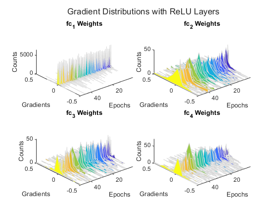
勾配分布のプロットを見ると、シグモイドネットワークがほとんど 0 に近い小さな勾配の影響を受けていることがわかります。この影響は、初期の層に向かって勾配がネットワーク内を逆伝播するほど顕著になります。

損失の比較

学習済みネットワークの損失を比較します。

figure
plot(losses)
xlabel("Iteration")
ylabel("Loss")
legend(activationTypes)

シグモイドネットワークの損失は、ReLU ネットワークの損失よりも緩やかに減少しています。そのため、このモデルの場合、ReLU 活性化層を使用したほうが高速に学習させることができます。

平均勾配の比較

各学習反復における各層の平均勾配を比較します。

figure
tiledlayout("flow")
for ii = 1:numLearnableLayers
    nexttile
    plot(meanGradients(:,:,ii))
    xlabel("Iteration")
    ylabel("Average Gradient")
    title(weightLayerNames(ii))
    legend(activationTypes)
end

平均勾配のプロットは、勾配分布のプロットで見られた結果と一致しています。シグモイド層を含むネットワークの場合、勾配の値は 0 を中心として非常に狭い範囲に分散しています。一方、ReLU 層を含むネットワークの場合、勾配はより広い範囲に分散しているため、勾配消失の可能性が減少して学習速度が増加します。

サポート関数

モデル損失関数

関数 modelLoss は、dlnetwork オブジェクト net、入力データ X のミニバッチ、およびラベルを含む対応するターゲット T を入力として受け取り、学習可能なパラメーターについての損失とその損失の勾配を返します。

function [loss,gradients] = modelLoss(net,X,T)
Y = forward(net,X);

loss = crossentropy(Y,T);
gradients = dlgradient(loss,net.Learnables);
end

ミニバッチ前処理関数

関数 preprocessMiniBatch は、次の手順を使用して予測子とラベルのミニバッチを前処理します。

関数 preprocessMiniBatchPredictors を使用してイメージを前処理します。
入力 cell 配列からラベルデータを抽出し、2 番目の次元に沿って categorical 配列にデータを連結します。
カテゴリカルラベルを数値配列に one-hot 符号化します。最初の次元への符号化は、ネットワーク出力の形状と一致する符号化された配列を生成します。

function [X,T] = preprocessMiniBatch(XCell,TCell)
% Preprocess predictors.
X = preprocessMiniBatchPredictors(XCell);

% Extract label data from cell and concatenate.
T = cat(2,TCell{1:end});

% One-hot encode labels.
T = onehotencode(T,1);
end

ミニバッチ予測子前処理関数

関数 preprocessMiniBatchPredictors は、入力 cell 配列からイメージデータを抽出して数値配列に連結することで、予測子のミニバッチを前処理します。グレースケール入力の場合、4 番目の次元で連結することにより、3 番目の次元が各イメージに追加されます。この次元は、大きさが 1 のチャネル次元として使用されます。

function X = preprocessMiniBatchPredictors(XCell)
% Concatenate.
X = cat(4,XCell{1:end});
end

分布の計算

関数 gradientDistributions は、ヒストグラムの値を計算し、ビンの中央値とヒストグラムのカウント数を返します。

function [centers,counts] = gradientDistributions(values)
% Get the histogram count for the values.
[counts,edges] = histcounts(values,30);

% histcounts returns edges of the bins. To get the bin centers,
% calculate the midpoints between consecutive elements of the edges.
centers =  edges(1:end-1) + diff(edges)/2;
end

勾配分布プロットの軸の作成

関数 setupGradientDistributionAxes は、勾配分布プロットを 3 次元でプロットするのに適した軸を作成します。この関数は、TiledChartLayout オブジェクトとカラーマップを含む構造体配列を返します。この構造体配列は、サポート関数 plotGradientDistributions への入力として機能します。

function plotSetup = setupGradientDistributionAxes(activationName,weightLayerNames,numEpochs)
f = figure;
t = tiledlayout(f,"flow",TileSpacing="tight");
t.Title.String = "Gradient Distributions with " + activationName + " Layers";

% To avoid updating the same values every epoch, set up axis 
% information before the training loop.
for i = 1 : numel(weightLayerNames)
    tiledAx = nexttile(t,i);

    % Set up the label names and titles.
    xlabel(tiledAx,"Gradients");
    ylabel(tiledAx,"Epochs");
    zlabel(tiledAx,"Counts");
    title(tiledAx,weightLayerNames(i));

    % Rotate the view.
    view(tiledAx, [-130, 50]);
    xlim(tiledAx,[-0.5,0.5]);
    ylim(tiledAx,[1,Inf]);
end

plotSetup.ColorMap = parula(numEpochs);
plotSetup.TiledLayout = t;
end

勾配分布のプロット

関数 plotGradientDistributions は、TiledChartLayout オブジェクトとカラーマップを含む構造体配列、および特定のエポックにおける値 (層の勾配など) から成る配列を入力として取り、平滑化されたヒストグラムを 3 次元でプロットします。適切な構造体配列の入力を生成するには、サポート関数 setupGradientDistributionAxes を使用します。

function plotGradientDistributions(plotSetup,gradientValues,epoch)

for w = 1:numel(gradientValues)
    nexttile(plotSetup.TiledLayout,w)
    color = plotSetup.ColorMap(epoch,:);

    values = extractdata(gradientValues{w});

    % Get the centers and counts for the distribution.
    [centers,counts] = gradientDistributions(values);

    % Plot the gradient values on the x axis, the epochs on the y axis, and the
    % counts on the z axis. Set the edge color as white to more easily distinguish
    % between the different histograms.
    hold("on");
    fill3(centers,zeros(size(counts))+epoch,counts,color,EdgeColor="#D9D9D9");
    hold("off")
    drawnow
end
end