Predict Shim Gaps from TDMS Data Using Machine Learning and Sensor Optimization

Since R2022a

This example shows how to reconstruct a spatial field of an aircraft using predictive shimming from sensor measurements stored in TDMS files.

Predictive shimming estimates a complete field from limited observations, reducing the need for dense sensor networks. The approach uses machine learning techniques such as Principal Component Analysis (PCA) to learn spatial patterns and QR pivoting to select the most informative sensor locations. Training models with this approach requires large datasets. TDMS files store and access large datasets efficiently because they are designed for high-volume, multi-channel measurement data.

In this example, you:

1. Load training data from TDMS files.

2. Compute a PCA basis to capture dominant spatial patterns.

3. Predict the spatial field using the PCA basis and optimal sensor locations.

4. Detect the saturation point where additional sensors yield minimal improvement.

5. Visualize reconstruction quality, sensor placement, and error trends.

6. Improve prediction accuracy by adjusting PCA parameters, sensor selection, or training data.

Load Training Data

In practice, collect the training data set by measuring the spatial field data for the aircraft region where the wing meets the fuselage. The spatial field data represents a displacement field that captures pointwise structural deformation across the wing–fuselage region.

For this example, load the provided aircraft data instead. The data consists of spatial field measurements of 20 aircraft, each represented on a 64-by-8 spatial grid. Each grid is flattened into a 512-by-1 vector and stored as a column in the TDMS file.

trainingTable = tdmsread("AircraftShimTraining.tdms");

tdmsread returns a cell array with one entry per channel group. The TDMS file used in this example contains the 20‑column training data set in a single channel group, so trainingTable{1} selects that table. Convert the table to a numeric array for easier processing.

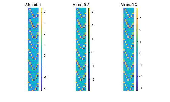
trainingData = table2array(trainingTable{1});

Visualize the training data set for three aircraft, converting each column back to its original 64-by-8 grid.

numRows = 64; numCols = 8;
figure(Name="Partial Training set");
for i = 1:3
    subplot(1,3,i);
    imagesc(reshape(trainingData(:,i),numRows,numCols));
    axis image off; 
    colorbar;
    title(sprintf("Aircraft %d",i));
end

Compute PCA Basis

Compute the dominant spatial patterns in the training data set using Principal Component Analysis (PCA). PCA identifies principal components to form a low-dimensional basis that captures most of the variance in the data.

The pcaBasis function provided with this example uses singular value decomposition (SVD), one of the standard methods for computing PCA. The basis obtained from this function captures 95% of the training variance. Increasing this threshold (for example, to 98%) includes more components in the basis, which can improve prediction accuracy. However, for large training data sets, the increase can lead to noticeably higher computation time.

pcaBasisMatrix = pcaBasis(trainingData,0.95);

PCA basis rank = 7

pcaBasis displays the resulting basis rank. In this case, the PCA analysis identifies seven components that capture 95% of the variance in the training data.

Predict with PCA and Sensor Selection

In addition to the training data, this example uses an independent spatial field measurement to test the predictive model. Load the spatial field for a single test aircraft.

testDataTable = tdmsread("AircraftShimTest.tdms");
testData = table2array(testDataTable{1});

To evaluate the trade-off between hardware complexity and prediction quality, vary the number of sensors and reconstruct the field using the PCA basis. The qrSensorSelection function provided with this example selects sensor locations using QR pivoting. The function then reconstructs the field using the PCA basis and computes the normalized reconstruction error. To improve reconstruction accuracy, use a different method to select sensor locations or reduce measurement noise.

noiseStd = 0.02;         
sensorCounts = 20:40:500;
[nmse,recons,sensors] = qrSensorSelection(pcaBasisMatrix,testData,sensorCounts,noiseStd);

Detect Saturation

Identify the sensor count where improvement in normalized mean square error (NMSE) becomes marginal. This count is the saturation point. This example computes successive improvements as sensor count increases and identifies the saturation point as the point where the improvement is less than 5%.

improvements = -diff(nmse) ./ nmse(1:end-1);
saturationIdx = find(improvements < 0.05, 1, "first") + 1;
if isempty(saturationIdx) 
    saturationSensorCount = sensorCounts(end);
    fprintf("Saturation not detected");
end
saturationSensorCount = sensorCounts(saturationIdx);
fprintf("Saturation detected at sensor count of %d\n", saturationSensorCount);

Saturation detected at sensor count of 100

Visualize Results

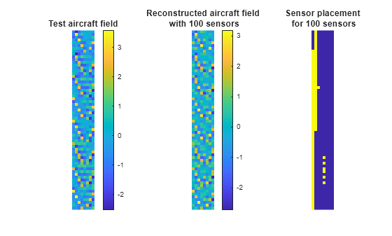
Compare the true and reconstructed fields of the test aircraft at the saturation point. Visualize the sensor layout, where yellow regions indicate sensor locations.

figure(Name="Reconstructed Field & Sensor Layout");
tiledlayout(1,3)

nexttile
imagesc(reshape(testData,numRows,numCols));
axis image off; 
colorbar;
title("Test aircraft field");

nexttile
imagesc(reshape(recons{saturationIdx},numRows,numCols));
axis image off;
colorbar;
title(sprintf("Reconstructed aircraft field\n with %d sensors",saturationSensorCount));

nexttile
mask = zeros(numRows*numCols,1);
mask(sensors{saturationIdx})=1;
imagesc(reshape(mask,numRows,numCols)); 
axis image off;
title(sprintf("Sensor placement\n for %d sensors",saturationSensorCount));

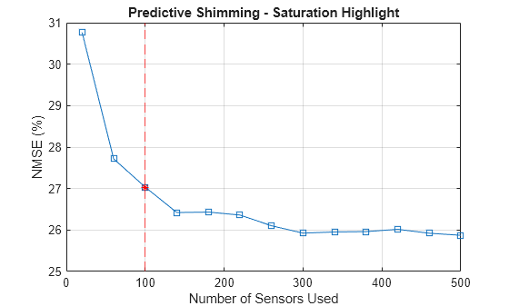
Plot NMSE versus sensor count and highlight the saturation point.

figure(Name="NMSE Saturation");
plot(sensorCounts,nmse*100,"-s");
hold on;
satX = sensorCounts(saturationIdx); satY = (nmse(saturationIdx))*100;
xline(satX,"r--");
plot(satX, satY, "r*");
hold off;
xlabel("Number of Sensors Used"); 
ylabel("NMSE (%)");
grid on;
title("Predictive Shimming - Saturation Highlight");

Improve Results

In this example, the NMSE at saturation is about 27%, which indicates that the prediction is not highly accurate. Improve accuracy by using more training data, reducing measurement noise, or increasing the PCA variance threshold to capture more spatial variability. Choosing a better method to select sensor locations can also help.

Try increasing the PCA variance threshold to 98% in the Compute PCA Basis section of this example. Then run the example to observe the impact on accuracy and saturation. When you increase the threshold from 95% to 98%, the PCA basis rank increases from 7 to 8, and the NMSE at saturation drops significantly from 27% to about 0.33%. Saturation now occurs at a sensor count of 140 instead of 100. This observation demonstrates the trade-off between accuracy, hardware complexity, and computation time.