Modal Truncation Model Reduction

Modal truncation method lets you discard poles based on their location or DC contribution. This method is useful when you want to focus your analysis on a particular subset of system dynamics. For instance, if you are working with a control system with bandwidth limited by actuator dynamics, you might discard higher-frequency dynamics in the plant. Eliminating dynamics outside the frequency range of interest reduces the numerical complexity of calculations with the model. There are two ways to compute a reduced-order model by mode selection:

• At the command line, using the reducespec workflow with "modal" method.

• In the Model Reducer, using the Modal Truncation method.

For more general information about model reduction, see Model Reduction Basics.

Modal Truncation in the Model Reducer App

Model Reducer provides an interactive tool for performing model reduction and examining and comparing the responses of the original and reduced-order models. To approximate a model by mode selection in Model Reducer:

1. Open the app and import an LTI model to reduce. For instance, suppose that there is a model named G in the MATLAB^® workspace. The following command opens Model Reducer and imports the model.

   modelReducer(G)

2. In the data browser, select the model to reduce. Click Modal Truncation.

   

   In the Modal Truncation tab, Model Reducer displays a plot of the frequency response of the original model and a reduced version of the model. The app also displays the pole locations of the original model.

   

   The plot marks pole locations with x.

   Note

   The frequency response is a Bode plot for SISO models, and a singular-value plot for MIMO models.

3. Model Reducer eliminates poles that lie outside the shaded region. Change the shaded region to capture only the dynamics you want to preserve in the reduced model. There are two ways to do so.

   • On either the response plot, drag the boundaries of the shaded region or the shaded region itself.

   • On the Modal Truncation tab, enter a model order reduction criteria based on frequency range, damping range, or the minimum DC contribution of modes.

   

   When you change the shaded regions or cutoff frequencies, Model Reducer automatically computes a new reduced-order model. All poles retained in the reduced model fall within the shaded region on the mode location plot. The reduced model might contain zeros that fall outside the shaded region.

   To customize the options, click Options. For more information, see Specify Options for Modal Truncation in Model Reducer.

4. Optionally, examine absolute or relative error between the original and simplified model. Select the error-plot type using the buttons on the Modal Truncation tab.

   

   For more information about using the analysis plots, see Visualize Reduced-Order Models in Model Reducer App.

5. When you have one or more reduced models that you want to store and analyze further, click Save Reduced Model. The new model appears in the data browser.

   

   After creating a reduced model in the data browser, you can continue adjusting the mode-selection region to create reduced models with different orders for analysis and comparison.

You can now perform further analysis with the reduced model. For example:

• Examine other responses of the reduced system, such as the step response or Nichols plot. To do so, use the tools on the Plots tab. See Visualize Reduced-Order Models in Model Reducer App for more information.

• Export reduced models to the MATLAB workspace for further analysis or control design. On the Model Reducer tab, click Export.

Generate MATLAB Code for Mode Selection

To create a MATLAB script you can use for further model-reduction tasks at the command line, click Save Reduced Model, and select Generate MATLAB Script.

Model Reducer creates a script that uses the reducespec and getrom commands to perform model reduction with the parameters you have set on the Mode Selection tab. The script opens in the MATLAB editor.

Modal Truncation at the Command Line

To reduce the order of a model by modal truncation at the command line, use reducespec. In this example, you reduce a high-order model with a focus on the dynamics in a particular frequency range and damping.

Load a model and examine its frequency response.

load('highOrderModel.mat','G')
bodeplot(G)

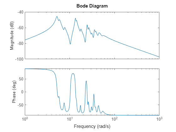
G is a 48th-order model with several large peak regions around 5.2 rad/s, 13.5 rad/s, and 24.5 rad/s, and smaller peaks scattered across many frequencies.

Create a model order reduction task.

R = reducespec(G,"modal");
view(R)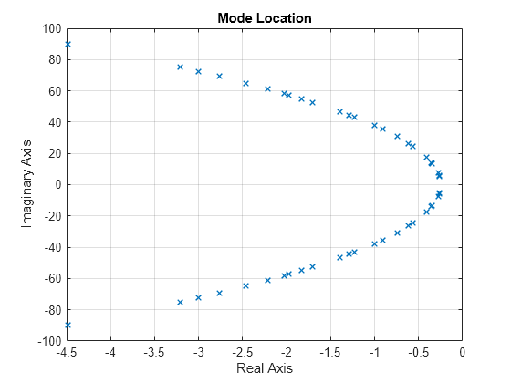

Suppose that for your application you are only interested in the dynamics between 10 rad/s and 40 rad/s with damping less than 0.04. Focus the model reduction on the region of interest to obtain a good match with a low-order approximation.

rsys = getrom(R,Frequency=[10,40],Damping=[0.022 0.04]);
opt = bodeoptions;
opt.PhaseMatching = "on";
bodeplot(G,rsys,"r--",opt)
legend("Full order","Reduced order")

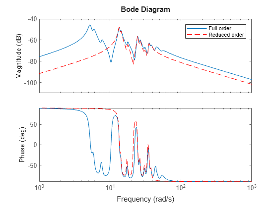
The reduced-order model provides a good approximation for the specified targets.