viewSurf
Visualize gain surface as a function of scheduling variables
Description
viewSurf( plots
the values of a 1-D or 2-D gain surface as a function of the scheduling
variables. GS)GS is a tunable gain surface that
you create with tunableSurface. The plot uses
the independent variable values specified in GS.SamplingGrid.
For 2-D gain surfaces, the design points in GS.SamplingGrid must
lie on a rectangular grid.
viewSurf(
plots the gain surface GS,xvar,xdata)GS at the scheduling-variable values
listed in xdata. The variable name xvar
must match a scheduling variable name in GS.SamplingGrid.
However, the values in xdata need not match design points in
GS.SamplingGrid.
For a 2-D gain surface, the plot shows a parametric family of
curves with one curve per value of the other scheduling variable.
In the 2-D case, the design points in GS.SamplingGrid must
lie on a rectangular grid.
viewSurf(
creates a surface plot of a 2-D gain surface evaluated over a grid of scheduling
variable values given by GS,xvar,xdata,yvar,ydata)ndgrid(xdata,ydata). In this case, the
design points of GS do not need to lie on a rectangular grid,
and xdata and ydata do not need to match
the design points.
Examples
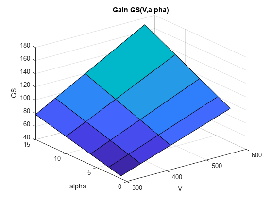
Display a tunable gain surface that depends on two independent variables.
Model a scalar gain K with a bilinear dependence on two scheduling variables, and V, as follows:
Here, x and y are the normalized scheduling variables. Suppose that is an angle of incidence that ranges from 0 degrees to 15 degrees, and V is a speed that ranges from 300 m/s to 600 m/s. Then, x and y are given by:
The coefficients are the tunable parameters of this variable gain. Use tunableSurface to model this variable gain.
[alpha,V] = ndgrid(0:1.5:15,300:30:600);
domain = struct('alpha',alpha,'V',V);
shapefcn = @(x,y) [x,y,x*y];
K = tunableSurface('K',1,domain,shapefcn);
Typically, you would tune the coefficients as part of a control system. You would then use setBlockValue or setData to write the tuned coefficients back to K, and view the tuned gain surface. For this example, instead of tuning, manually set the coefficients to non-zero values and view the resulting gain.
Ktuned = setData(K,[100,28,40,10]);
viewSurf(Ktuned)
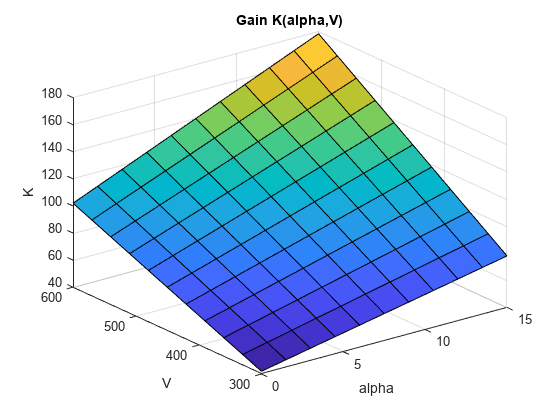
viewSurf displays the gain surface as a function of the scheduling variables, for the ranges of values specified by domain and stored in Ktuned.SamplingGrid.
View a 1-D gain surface evaluated at different design points from the points specified in the gain surface.
When you create a gain surface using tunableSurface, you specify design points at which the gain coefficients are tuned. These points are the typically the scheduling-variable values at which you have sampled or linearized the plant. However, you might want to implement the gain surface as a lookup table with breakpoints that are different from the specified design points. In this example, you create a gain surface with a set of design points and then view the surface using a different set of scheduling variable values.
Create a scalar gain that varies as a quadratic function of one scheduling variable, t. Suppose that you have linearized your plant every five seconds from t = 0 to t = 40.
t = 0:5:40;
domain = struct('t',t);
shapefcn = @(x) [x,x^2];
GS = tunableSurface('GS',1,domain,shapefcn);
Typically, you would tune the coefficients as part of a control system. For this example, instead of tuning, manually set the coefficients to non-zero values.
GS = setData(GS,[12.1,4.2,2]);
Plot the gain surface evaluated at a different set of time values.
tvals = [0,4,11,18,25,32,39,42];
viewSurf(GS,'t',tvals)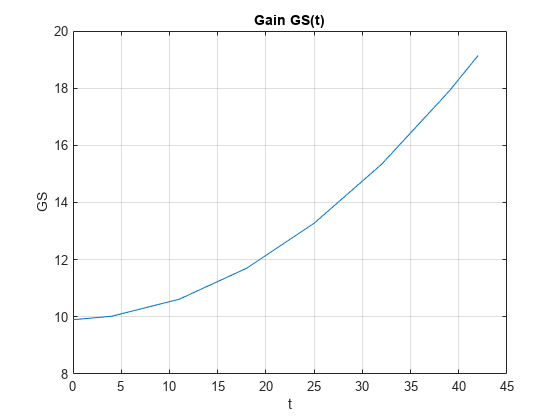
The plot shows that the gain curve bends at the points specified in tvals, rather than the design points specified in domain. Also, tvals includes values outside of the scheduling-variable range of domain. If you attempt to extrapolate too far out of the range of values used for tuning, the software issues a warning.
Plot gain surface values as a function of one independent variable, for a gain surface that depends on two independent variables.
Create a gain surface that is a bilinear function of two independent variables, and V.
[alpha,V] = ndgrid(0:1.5:15,300:30:600);
domain = struct('alpha',alpha,'V',V);
shapefcn = @(x,y) [x,y,x*y];
GS = tunableSurface('GS',1,domain,shapefcn);
Typically, you would tune the coefficients as part of a control system. For this example, instead of tuning, manually set the coefficients to non-zero values.
GS = setData(GS,[100,28,40,10]);
Plot the gain at selected values of V.
Vplot = [300:50:600];
viewSurf(GS,'V',Vplot);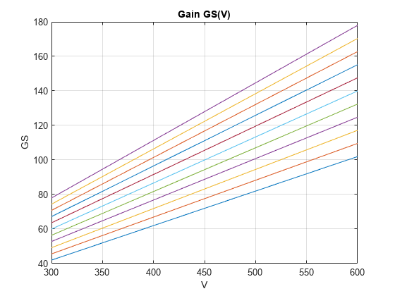
viewSurf evaluates the gain surface at the specified values of V, and plots the dependence on V for all values of in domain. Clicking any of the lines in the plot displays the corresponding value. This plot is useful to visualize the full range of gain variation due to one independent variable.
View a 2-D gain surface evaluated at different scheduling-variable values from the design points specified in the gain surface.
When you create a gain surface using tunableSurface, you specify design points at which the gain coefficients are tuned. These points are typically the scheduling-variable values at which you have sampled or linearized the plant. However, you might want to implement the gain surface as a lookup table with breakpoints that are different from the specified design points. In this example, you create a gain surface with a set of design points and then view the surface using a different set of scheduling-variable values.
Create a gain surface that is a bilinear function of two independent variables, and V.
[alpha,V] = ndgrid(0:1.5:15,300:30:600);
domain = struct('alpha',alpha,'V',V);
shapefcn = @(x,y) [x,y,x*y];
GS = tunableSurface('GS',1,domain,shapefcn);
Typically, you would tune the coefficients as part of a control system. For this example, instead of tuning, manually set the coefficients to non-zero values.
GS = setData(GS,[100,28,40,10]);
Plot the gain at selected values of and V.
alpha_vec = [7:1:13];
V_vec = [500:25:625];
viewSurf(GS,'alpha',alpha_vec,'V',V_vec);
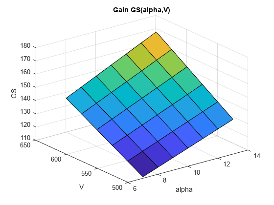
The breakpoints at which you evaluate the gain surface need not fall within the range specified by domain. However, if you attempt to evaluate the gain too far outside the range used for tuning, the software issues a warning.
The breakpoints also need not be regularly spaced. In addition, you can specify the scheduling variables in any order to get a different perspective on the shape of the surface. The variable that you specify first is used as the X-axis in the plot.
alpha_vec2 = [1,3,6,10,15];
V_vec2 = [300,350,425,575];
viewSurf(GS,'V',V_vec2,'alpha',alpha_vec2);
Input Arguments
Version History
Introduced in R2015b