このページの内容は最新ではありません。最新版の英語を参照するには、ここをクリックします。

パワー アンプのバックオフのシミュレーションと検証

この例では、バックオフを使用して、信号をテーブルに基づくパワー アンプに入力する前にスケーリングする方法を説明します。また、アンプへの信号入力のパワー分布を調べる方法と、アンプの実際の動作が仕様に一致していることを検証する方法も説明します。この例で使用される補助関数のリストは付録にあります。

システム設定

M = 16;             % Modulation order
fs = 1e6;           % Sample rate in Hz & measurement bandwidth
sigDuration = 0.01; % sec
msgLen = round(sigDuration*fs); % Number of samples
totalTime = 0;

アンプをテーブルに基づくオブジェクトとして指定します。Excel スプレッドシートに格納された計測されたアンプ データを使用して、出力パワーと入力パワーの比較、および位相の変化と入力パワーの比較を読み取ります。パワーは dBm 単位で与えられ、位相の変化は度単位で与えられます。基準インピーダンスは信号の電圧の値を電力の値に変換するために使用されます。

table = table2array(readtable( ...
    "PACharacteristic.xlsx", ...
    PreserveVariableNames=true));
mnl = comm.MemorylessNonlinearity( ...
    Method="Lookup table", ...
    Table=table, ...
    ReferenceImpedance=1);

結果としてピーク出力パワーとなる入力パワーを決定します。その入力パワーは、そこから信号がバックオフされる点です。入力バックオフを使用して、アンプへの入力で必要な信号パワーを決定します。

[pkOpPwr, idxPk] = max(mnl.Table(:,2)); % dBm
ipPwrAtPkOut = mnl.Table(idxPk,1);      % dBm
IBO = 6;                                % input backoff set point, dB
rqdIpPwr = ipPwrAtPkOut - IBO;          % dBm

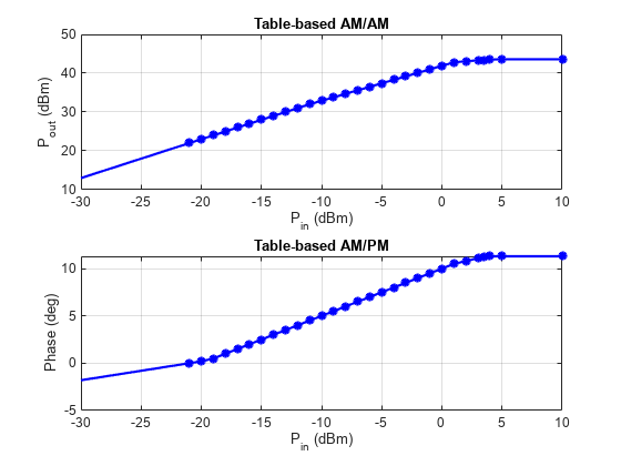
AM/AM アンプ特性と AM/PM アンプ特性をプロットします。プロットされる値はスプレッドシートの値と一致しています。

plot(mnl);

システム シミュレーションと検証

パルス整形のためのレイズド コサイン送信フィルター System object を作成します。

txFilt = comm.RaisedCosineTransmitFilter( ...
  Shape='Square root', ...
  RolloffFactor=0.2, ...
  FilterSpanInSymbols=10, ...
  OutputSamplesPerSymbol=4);

パワー メーター System object を作成して処理チェーンの複数の点でパワーを測定します。パワー メーターの測定ウィンドウを 10 ms に設定します。

pm = powermeter(...
  Measurement="Average power", ...
  WindowLength=round(sigDuration*fs), ...
  ReferenceLoad=mnl.ReferenceImpedance, ...
  PowerUnits="dBm");

変調された信号を生成し、それをフィルター処理し、-10 dBm にスケーリングして、パワーを測定します。フィルター処理された信号はその持続時間を通じてほぼ一定の振幅であり、そのためパワー測定ウィンドウは持続時間全体に延びる可能性があります。

filtTransient = ...
    txFilt.FilterSpanInSymbols*txFilt.OutputSamplesPerSymbol;
msg = randi([0 M-1],msgLen+filtTransient,1);
modOut = qammod(msg,M, ...
    UnitAveragePower=true);             % 0 dBW (30 dBm)
filtOut = txFilt(modOut);
filtOut = filtOut(1+filtTransient:end); % Truncate beginning transient
PFiltOutdBm = pm(filtOut);
Pdesired = -10;  % dBm
scaleFactor = 10.^((Pdesired - PFiltOutdBm(end))/20);
filtOut = scaleFactor * filtOut;
reset(pm);
PFiltOutdBm = pm(filtOut);
fprintf('The filtered, scaled signal power is %4.2f dBm.\n', ...
    PFiltOutdBm(end))

The filtered, scaled signal power is -10.00 dBm.

PFiltOutdBW = PFiltOutdBm(end) - 30;

アンプ入力パワーを目的のバックオフにスケーリングします。バックオフした信号の測定されたパワーは、ピーク出力 (5 dBm) での入力パワーから入力バックオフ (6 dB) を引いたものと等しくなければなりません。パワー メーターにより、信号が適切にバックオフされていることが検証されます。

gain = helperBackoffGain(ipPwrAtPkOut,PFiltOutdBm(end),IBO);
ampIn = gain * filtOut;
reset(pm);
PAmpIndBm = pm(ampIn);
fprintf('The backed off signal power is %4.2f dBm.\n', ...
    PAmpIndBm(end))

The backed off signal power is -1.00 dBm.

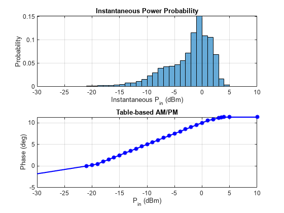
アンプへの瞬時の入力パワーのヒストグラムをプロットします。次の図は、アンプの入力サンプルの相当の割合が、アンプ出力でゲイン圧縮を引き起こすパワーとなっていることを示しています。多くの信号サンプルが 0 dBm を上回るパワーとなっており、そこではアンプは非線形に動作します。

PAmpInInst = abs(ampIn).^2 / mnl.ReferenceImpedance;
PAmpInInstdBm = 10*log10(PAmpInInst) + 30;
edges = -29:9;
histogram(PAmpInInstdBm,edges,Normalization="probability")
title("Instantaneous Power Probability");
xlabel("Instantaneous P_i_n (dBm)");
ylabel("Probability");
xlim([-30 10]);
grid on;

アンプを通じて信号を渡します。アンプの出力での測定された平均パワーは、前の図で示された、想定される瞬時電力と密接に対応しています。

ampOut = mnl(ampIn);
PAmpOutdBm = pm(ampOut);
fprintf('The amplifier output power is %4.2f dBm.\n', ...
    PAmpOutdBm(end))

The amplifier output power is 40.63 dBm.

アンプのゲインの平均を計算します。

ampGaindB = PAmpOutdBm(end) - PAmpIndBm(end);
fprintf('The amplifier gain is %4.2f dB.\n', ...
    ampGaindB)

The amplifier gain is 41.63 dB.

指定されたものと実際の瞬時の $$P_{\text{out}}$$ と $$P_{\text{in}}$$ をプロットして、アンプの実際の動作が、テーブルに基づくオブジェクトで指定された動作と一致することを示します。

figure;
hFig = helperPlotAMAM(mnl); % Specified Pout vs. Pin
hold on;
pAmpOutInst = abs(ampOut).^2 / mnl.ReferenceImpedance;
pAmpOutInstdBm = 10*log10(pAmpOutInst) + 30;  % Actual Pout vs Pin
plot(PAmpInInstdBm,pAmpOutInstdBm,'r*');
grid on;
lines = hFig.Children.Children;
legend(lines([2 1]),Specified="Actual",Location="Northwest");

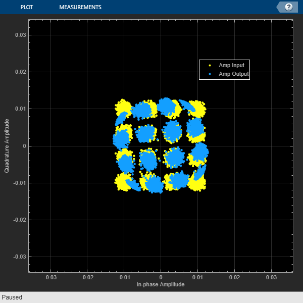
コンスタレーション ダイアグラムを作成して、アンプの入力信号と出力信号を示します。16QAM コンスタレーションのコンスタレーション ダイアグラムは、アンプ出力が少し回転 (AM/PM 歪み) しており、コーナー ポイントには若干のゲイン圧縮が発生 (AM/AM 歪み) していることを示しています。

constDiag = comm.ConstellationDiagram( ...
  ShowReferenceConstellation=false, ...
  SamplesPerSymbol=txFilt.OutputSamplesPerSymbol, ...
  ShowLegend=true, ...
  ChannelNames={'Amp Input','Amp Output'});

% Set plot limits
maxLim = 2 * max(real(filtOut));
constDiag.XLimits = [-maxLim maxLim];
constDiag.YLimits = [-maxLim maxLim];

magFiltOut = sqrt(mean(abs(filtOut).^2));
magAmpOut = sqrt(mean(abs(ampOut).^2));
gain = magAmpOut / magFiltOut;
constDiag([filtOut,ampOut/gain]); % Scale amp output for plotting ease

例の検証

この例で、異なるバックオフ レベルや変調された信号 (たとえば 64QAM や OFDM) を試して、実験することができます。独自のテーブルに基づく $P_{\text{out}}\text{vs.}{P}_{\text{in}}$ 特性を含むスプレッドシートを読み込んで、このバックオフ手法を自身の PA 特性に適用できます。

まとめ

この例では、非線形アンプの入力信号にバックオフを適用する方法を説明しました。この手法は、指定されたデータと実際のデータの$P_{\text{out}}\text{vs.}{P}_{\text{in}}$ の動作を比較することで検証されました。

付録

この例では、次の補助ファイルが使用されています。

• helperBackoffGain.m

• helperPlotAMAM.m