plot
Display RF propagation rays in Site Viewer
Description
plot(
displays the rays using additional options specified by name-value arguments.rays,Name=Value)
Examples
Perform ray tracing in Chicago and return the rays in comm.Ray objects. Then, display the rays without performing the ray tracing analysis again.
Launch Site Viewer with buildings in Chicago. For more information about the OpenStreetMap® file, see [1].
viewer = siteviewer(Buildings="chicago.osm");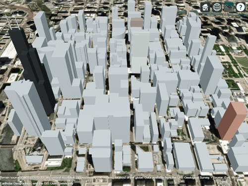
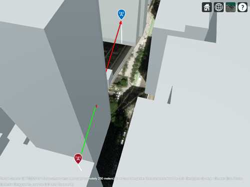
Create a transmitter site on one building and a receiver site on another building. Show the line-of-sight path between the sites using the los function.
tx = txsite(Latitude=41.8800, ...
    Longitude=-87.6295, ...
    TransmitterFrequency=2.5e9);
rx = rxsite(Latitude=41.881352, ...
    Longitude=-87.629771, ...
    AntennaHeight=30);
los(tx,rx)
Create a ray tracing propagation model, which MATLAB® represents using a RayTracing object. By default, the model uses the SBR method and calculates propagation paths with up to two reflections.
pm = propagationModel("raytracing");Perform the ray tracing analysis. The raytrace function returns a cell array containing the comm.Ray objects.
rays = raytrace(tx,rx,pm)
rays = 1×1 cell array
    {1×3 comm.Ray}
View the properties of the first ray object.
rays{1}(1)ans =
Ray with properties:
PathSpecification: 'Locations'
CoordinateSystem: 'Geographic'
TransmitterLocation: [3×1 double]
ReceiverLocation: [3×1 double]
LineOfSight: 0
Interactions: [1×1 struct]
Frequency: 2.5000e+09
PathLossSource: 'Custom'
PathLoss: 92.7686
PhaseShift: 1.2945
Read-only properties:
PropagationDelay: 5.7088e-07
PropagationDistance: 171.1462
AngleOfDeparture: [2×1 double]
AngleOfArrival: [2×1 double]
NumInteractions: 1
Close Site Viewer.
close(viewer)
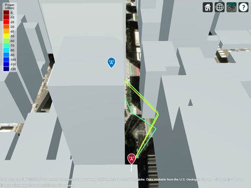
Create another Site Viewer with the same buildings, transmitter site, and receiver site. Then, display the propagation paths. Alternatively, you can plot individual paths by specifying a single ray object, for example rays{1}(2).
siteviewer(Buildings="chicago.osm");
show(tx)
show(rx)
plot(rays{1},Type="power", ...
    TransmitterSite=tx,ReceiverSite=rx)
Appendix
[1] The OpenStreetMap file is downloaded from https://www.openstreetmap.org, which provides access to crowd-sourced map data all over the world. The data is licensed under the Open Data Commons Open Database License (ODbL), https://opendatacommons.org/licenses/odbl/.
Input Arguments
Name-Value Arguments
Version History
Introduced in R2020a
1 Alignment of boundaries and region labels are a presentation of the feature provided by the data vendors and do not imply endorsement by MathWorks®.