Train 3-D Speech Enhancement Network Using Deep Learning

This example uses:

In this example, you train a filter and sum network (FaSNet) [1] to perform speech enhancement (SE) using ambisonic data. The model has been updated to use stacked dual-path recurrent neural networks (DPRNNs) which enable memory-efficient joint modeling of short- and long-term sequences [4]. To explore the model trained in this example, see 3-D Speech Enhancement Using Trained Filter and Sum Network.

Introduction

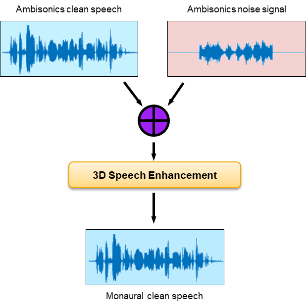
The aim of speech enhancement (SE) is to suppress the noise in a noisy speech signal. The SE system may be used as a front end in teleconferencing systems, where intelligibility and listening experience are important metrics, or a speech-to-text system, where the word error rate of the downstream speech-to-text system is the important metric.

In this example, you use the L3DAS 2021 Task 1 dataset [2] to train and evaluate a model that uses B-format ambisonic data to perform speech enhancement. The enhanced speech is output as a mono audio signal. To explore the model trained in this example, see 3-D Speech Enhancement Using Trained Filter and Sum Network.

Optionally Reduce Data Set

To train the network with the entire data set, set speedupExample to false. To run this example quickly, set speedupExample to true. This network requires a large amount of data to achieve reasonable results.

speedupExample = false;

Download and Prepare Data

This example uses the L3DAS21 task 1 challenge data set [2]. The train data sets contains 2 multiple-source and multiple-perspective (MSMP) B-format ambisonic recordings collected at a sampling rate of 16 kHz. The two microphones are labeled as "A" and "B". In this example, you discard recordings from microphone B. Including microphone B data in the training should improve the final performance. The train and validation splits are provided with the data set. The 3-D speech enhancement data set contains more than 30,000 virtual 3-D audio environments with a duration up to 10 seconds. Each sample contains a spoken voice and other office-like background noises. The target data is the clean monophonic voice signal. The dev dataset is 2.6 GB, the train100 dataset is 7.6 GB, and the train360 dataset is 28.6 GB.

Download the data set and point to it using audioDatastore.

downloadLocation = tempdir;

datasetLocationDev = fullfile(downloadLocation,"L3DAS_Task1_dev");
datasetLocationTrain100 = fullfile(downloadLocation,"L3DAS_Task1_train100");
datasetLocationTrain360 = fullfile(downloadLocation,"L3DAS_Task1_train360");
if speedupExample
    if ~datasetExists(datasetLocationDev)
        urlDev = "https://zenodo.org/record/4642005/files/L3DAS_Task1_dev.zip";
        unzip(urlDev,downloadLocation)
    end

    ads = audioDatastore(fullfile(downloadLocation,"L3DAS_Task1_dev"),IncludeSubfolders=true);
else
    if ~datasetExists(datasetLocationDev)
        urlDev = "https://zenodo.org/record/4642005/files/L3DAS_Task1_dev.zip";
        unzip(urlDev,downloadLocation)
    end
    if ~datasetExists(datasetLocationTrain100)
        urlTrain100 = "https://zenodo.org/record/4642005/files/L3DAS_Task1_train100.zip";
        unzip(urlTrain100,downloadLocation)
    end
    if ~datasetExists(datasetLocationTrain360)
        urlTrain360 = "https://zenodo.org/record/4642005/files/L3DAS_Task1_train360.zip";
        unzip(urlTrain360,downloadLocation)
    end
    adsValidation = audioDatastore(fullfile(downloadLocation,"L3DAS_Task1_dev"),IncludeSubfolders=true);
    adsTrain = audioDatastore([fullfile(downloadLocation,"L3DAS_Task1_train100"), ...
        fullfile(downloadLocation,"L3DAS_Task1_train360")],IncludeSubfolders=true);
end

To subset the datastores into targets and predictors, use subset. Only use microphone A predictors. Using both microphones should increase model performance at the cost of more training time.

if speedupExample
    [~,fileNames] = fileparts(ads.Files);
    targetFiles = ~endsWith(fileNames,["A","B"]);
    micAFiles = endsWith(fileNames,"A");
    T = subset(ads,targetFiles);
    X = subset(ads,micAFiles);
    XTrain = subset(X,1:40);
    TTrain = subset(T,1:40);
    XValidation = subset(X,41:50);
    TValidation = subset(T,41:50);
else
    [~,fileNames] = fileparts(adsTrain.Files);
    targetFiles = ~endsWith(fileNames,["A","B"]);
    micAFiles = endsWith(fileNames,"A");
    TTrain = subset(adsTrain,targetFiles);
    XTrain = subset(adsTrain,micAFiles);

    [~,fileNames] = fileparts(adsValidation.Files);
    targetFiles = ~endsWith(fileNames,["A","B"]);
    micAFiles = endsWith(fileNames,"A");
    TValidation = subset(adsValidation,targetFiles);
    XValidation = subset(adsValidation,micAFiles);
end

Remove any files that do not overlap between targets and predictors.

[~,hFiles] = fileparts(TTrain.Files);
[~,kFiles] = fileparts(XTrain.Files);
kFiles = erase(kFiles,"_A");
validFiles = intersect(kFiles,hFiles);
targetValidFiles = ismember(validFiles,kFiles);
predictorsValidFiles = ismember(kFiles,validFiles);
TTrain = subset(TTrain,targetValidFiles);
XTrain = subset(XTrain,predictorsValidFiles);

[~,hFiles] = fileparts(TValidation.Files);
[~,kFiles] = fileparts(XValidation.Files);
kFiles = erase(kFiles,"_A");
validFiles = intersect(kFiles,hFiles);
targetValidFiles = ismember(validFiles,kFiles);
predictorsValidFiles = ismember(kFiles,validFiles);
TValidation = subset(TValidation,targetValidFiles);
XValidation = subset(XValidation,predictorsValidFiles);

To combine the predictor and target datastores so that reading from the combined datastore returns the predictors and associated target, use combine.

dsTrain = combine(XTrain,TTrain);
dsValidation = combine(XValidation,TValidation);

Inspect Data

Preview the ambisonic recordings and plot the data.

predictor = preview(XTrain);
target = preview(TTrain);

fs = 16e3; % Known sampling rate of data.
t = (0:size(target,1)-1)/fs;

tiledlayout(2,1,TileSpacing="tight")

nexttile
plot(t,target)
title("Target")
xlabel("Time (s)")
axis tight

nexttile
plot(t,predictor)
title("Predictor")
xlabel("Time (s)")
legend(["W","X","Y","Z"])
axis tight

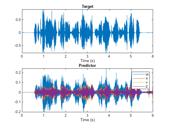
Listen to the target data, the mean of the ambisonic channels, or one of the ambisonic channels individually.

soundSource = predictor(:,1);
soundsc(soundSource,fs)

Word Error Rate (WER)

Choosing an appropriate metric to evaluate a SE system performance depends on the final task of the system. For speech-to-text applications, evaluating the word error rate (WER) using the target speech-to-text system is a common approach. For teleconferencing applications, the short-time objective intelligibility measure (STOI) is a common approach. Similarly, the choice of loss function should depend on the final application of the speech enhancement system. In this example, you attempt to optimize the system to reduce WER for a downstream speech-to-text system. One option for the loss function is to use the WER directly, however this can be prohibitively time-consuming for training, and couples the speech enhancement module tightly with the speech-to-text module. Another approach is to use an auditory-based representation of the targets and predictors and calculate the mean square error between them. This example takes the second approach. To get a baseline for performance analysis, calculate the WER of the target (clean) signal, and the noisy signal using a naive approach to SE (mean over channels). The supporting function, wordErrorRate, uses the wav2vec2.0 option of the speech2text functionality. If you have not downloaded the pretrained wav2vec 2.0 model, the function throws an error with a link to the download. The WER is calculated using Text Analytics Toolbox™.

tds = fileDatastore(datasetLocationDev, ...
    ReadFcn=@(x)string(fileread(x)), ...
    IncludeSubfolders=true,FileExtensions=".txt");
[~,tdsFiles] = fileparts(tds.Files);
[~,TValidationFiles] = fileparts(TValidation.Files);
validFiles = ismember(tdsFiles,TValidationFiles);
tds = subset(tds,validFiles);
dsWER = combine(XValidation,TValidation,tds);

WERa = wordErrorRate(dsWER,TargetWER=true,BaselineWER=true);

progress = 1.2.3.4.5.6.7.8.9.10.11.12.13.14.15.16.17.18.19.20.21.22.23.24.25.26.27.28.29.30.31.32.33.34.35.36.37.38.39.40.41.42.43.44.45.46.47.48.49.50.51.52.53.54.55.56.57.58.59.60.61.62.63.64.65.66.67.68.69.70.71.72.73.74.75.76.77.78.79.80.81.82.83.84.85.86.87.88.89.90.91.92.93.94.95.96.97.98.99....complete.

WERa.Target

ans = 0.0296

WERa.Baseline

ans = 0.4001

Filter and Sum Network (FaSNet)

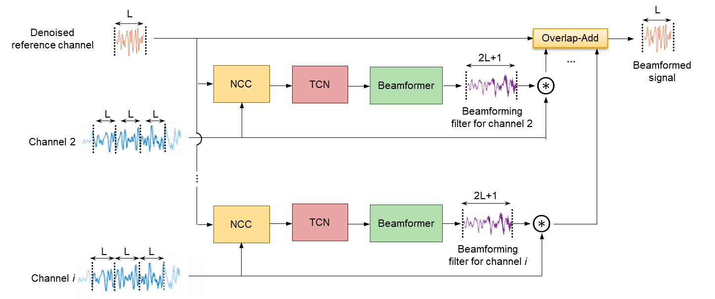
This example uses the filter and sum network (FaSNet) architecture with dual-path recurrent neural networks (DPRNN). FaSNet is a time-domain adaptive beamforming framework consisting of two stages:

Estimate the beamforming filter for selected reference channel, and then denoise the reference signal.
Beamform remaining channels using the denoised reference channel.

The FaSNet using DPRNN architecture is implemented in the supporting function FaSNet, which is in the current folder when you open this example.

Stage 1: Denoise Reference Mic

In stage one, a normalized cross correlation (NCC) metric is computed between the windows of the reference channel with context and windows of the remaining channels. This example uses cosine similarity as the correlation metric. The metric is pooled across the channels, passed through a temporal convolutional network (TCN), and then through the beamforming filter learner. The output from the beamformer module blocks is then used to filter the reference channel.

Stage 2: Create Beamformed Signal

In stage two, a NCC metric is computed between the denoised windows of the reference channel and windows of the remaining channels with context. A beamforming filter is learned for each of the remaining channels. Each channel is separately denoised, and then the channels are summed to create the beamformed final signal.

Beamformer

The beamformer module follows the design of [1] except replaces the stacked TCN blocks with stacked DPRNN blocks.

Dual-Path Recurrent Neural Network

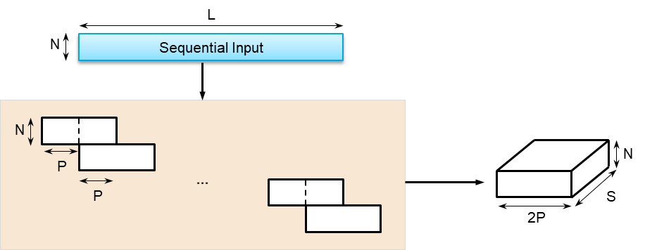
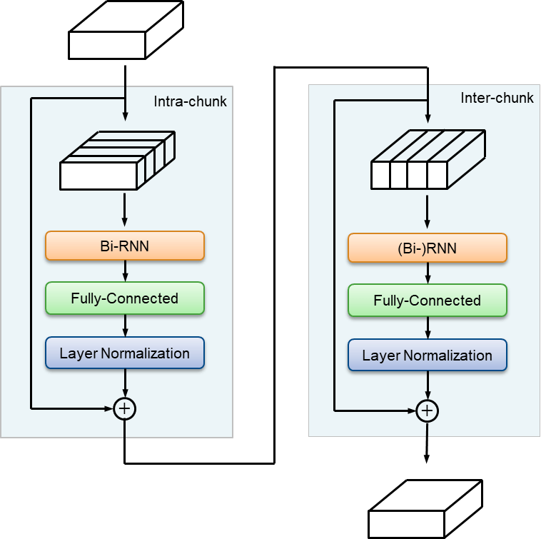
Dual-path recurrent neural networks (DPRNN) were introduced in [4] as a method of organizing RNN layers in a deep structure to model extremely long sequences. DPRNN splits sequential input into chunks and then applies intra- and inter-chunk operations iteratively. The approach has been shown to perform as well or better than 1-D CNN architectures with a significantly smaller model size. The DPRNN model consists of three stages: segmentation, DPRNN blocks (which may be stacked), and then overlap-add reconstruction.

Segmentation

The sequence is split into S segments of length K with overlap P. In this example, K = 2P.

DPRNN Block

The segmented signal passes through B DPRNN blocks. In this example, B is set to 6. Each block contains two sub-modules corresponding to intra- and inter-chunk processing. The intra-chunk RNN is always bi-directional. The intra-chunk RNN processes each segment individually. The inter-chunk RNN may be uni- or bi-directional, depending on latency requirements of your system. In this example, the inter-chunk RNN is bi-directional. The inter-chunk RNN processes along the stacked dimension of length S. The output of each DPRNN block is the same size as the input.

Overlap-Add

The output from the stacked DPRNN blocks is overlapped and added to reconstruct the sequence data.

Define Parameters

Define system-level, FaSNet-level, and DPRNN-level parameters.

% System-level parameters
parameters.SampleRate = fs;
parameters.AnalysisLength = 2*parameters.SampleRate;

% FaSNet-level parameters
parameters.WindowLength = 256;    % L in FaSNet
parameters.EncoderDimension = 64; % Number filters in TCN
parameters.NumDPRNNBlocks = 6;    % Number of stacked DPRNN blocks

% DPRNN-level parameters
parameters.FeatureDimension = 64; % Number of filters in convolutional blocks
parameters.SegmentSize = 24;      % 2P
parameters.HiddenDimension = 128; % RNN size

Initialize Network Learnables

Use the supporting function, intitializeLearnables, to initialize the FaSNet architecture for the specified parameters.

learnables = initializeLearnables(parameters);

Input Pipeline

Define the mini-batch size. Create minibatchqueue (Deep Learning Toolbox) objects to read mini-batches from the training data set. The supporting function preprocessMiniBatch randomly selects a single clip of the specified parameters.AnalysisLength from each audio file in the mini-batch. This approach avoids the need to buffer and save individual audio files, which reduces disk space requirements. The approach has the added benefit of changing the exact sequences seen between epochs. However, this approach puts more emphasis on shorter files in the training data.

miniBatchSize = 32;

mbqTrain = minibatchqueue(dsTrain, ...
    MiniBatchSize=miniBatchSize, ...
    MiniBatchFcn=@(x,t)preprocessMiniBatch(x,t,parameters.AnalysisLength), ...
    DispatchInBackground=canUseParallelPool && ~speedupExample);

mbqValidation = minibatchqueue(dsValidation, ...
    MiniBatchSize=miniBatchSize, ...
    MiniBatchFcn=@(x,t)preprocessMiniBatch(x,t,parameters.AnalysisLength), ...
    DispatchInBackground=canUseParallelPool && ~speedupExample);

Training Options

Choose a loss metric as auditory-mse, sample-mse, or sample-sisdr.

auditory-mse: Use the mean-square-error (MSE) between a mel spectrogram computed from the target and a mel spectrogram computed from the prediction.
sample-mse: Use the sample-level MSE between the target and predictor.
sample-sisdr: Use the sample-level scale-invariant signal-to-distortion ratio defined in [3].

lossType = "auditory-mse";

Define the maximum number of epochs, the initial learn rate, and piece-wise learning parameters such as validation patience, learn rate drop factor, and minimum learn rate. The default settings correspond to those reported in [4] for the task of speaker separation.

maxEpochs = 100;
initialLearnRate = 0.001;
validationPatience = 10;
learnRateDropFactor = 0.98;
learnRateDropPeriod = 2;

if speedupExample
    maxEpochs = 1;
end

Initialize parameters required for the training loop.

iteration = 0;
bestLoss = inf;
averageGrad = [];
averageSqGrad = [];
learnRate = initialLearnRate;

Train Network

Create a trainingProgressMonitor to monitor the training loss and validation loss while training.

monitor = trainingProgressMonitor( ...
    Metrics=["TrainingLoss","ValidationLoss"], ...
    Info=["Epoch","LearnRate"]);
groupSubPlot(monitor,"Loss",["TrainingLoss","ValidationLoss"])

Record the loss for the untrained network.

validationLoss = mbqLoss(mbqValidation,learnables,parameters,lossType);
recordMetrics(monitor,0,ValidationLoss=validationLoss)

Run the training loop.

for epoch = 1:maxEpochs

    % Update plot info
    updateInfo(monitor,Epoch=epoch,LearnRate=learnRate)

    % Shuffle dataset each epoch
    shuffle(mbqTrain)

    while hasdata(mbqTrain)
        iteration = iteration + 1;

        % Get next mini batch
        [X,T] = next(mbqTrain);

        % Pass the predictors through the network and return the loss and
        % gradients.
        [loss,gradients] = dlfeval(@modelLoss,learnables,parameters,X,T,lossType);

        % Update the network parameters using the ADAM optimizer.
        [learnables,averageGrad,averageSqGrad] = adamupdate(learnables,gradients, ...
            averageGrad,averageSqGrad,iteration,learnRate);

        % Update training progress visualization
        loss = gather(extractdata(loss));
        recordMetrics(monitor,iteration,TrainingLoss=loss)

        if monitor.Stop
            break
        end
    end
    if monitor.Stop
        break
    end

    % Compute validation loss
    validationLoss = mbqLoss(mbqValidation,learnables,parameters,lossType);

    % Update validation progress visualization
    recordMetrics(monitor,iteration,ValidationLoss=validationLoss)

    % Checkpoint
    if validationLoss < bestLoss
        bestLoss = validationLoss;
        bestLossEpoch = epoch;
        save("CheckPoint.mat","bestLoss","learnables","epoch", ...
            "averageGrad","averageSqGrad","iteration","learnRate")
    end

    if (epoch - bestLossEpoch) > validationPatience
        display("Validation loss did not improve for "+validationPatience+" epochs.")
        break
    end

    % Reduce the learning rate according to schedule
    if rem(epoch,learnRateDropPeriod)==0
        learnRate = learnRate*learnRateDropFactor;
    end
end

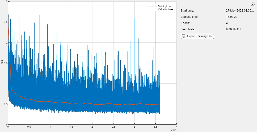
    "Validation loss did not improve for 10 epochs."

Evaluate System

Load the best performing model.

load("CheckPoint.mat")

Spot Check Performance

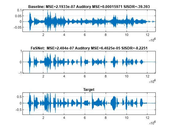
Compare the results of the baseline speech enhancement approach against the FaSNet approach using listening tests and common metrics.

dsValidation = shuffle(dsValidation);
[x,t] = read(dsValidation);
predictor = x{1};
target = x{2};

As a baseline speech enhancement system, simply take the mean of the predictors across the channels.

yBaseline = mean(predictor,2);

Pass the noisy speech through the network. The network was trained to process data in 2-second segments. The architecture does accept longer and shorter segments, but performs best on inputs of the same size as it was trained on. Use the preprocessSignal supporting function to split the audio input into the same segment length as your model was trained on. Pass the segments through the FaSNet model. Treat each segment individually by placing the segment dimension along the third dimension, which the FaSNet model recognizes as the batch dimension.

y = preprocessSignal(predictor,parameters.AnalysisLength);

y = FaSNet(dlarray(y),parameters,learnables);

y = gather(extractdata(y)); % Convert to regular array
y = y(:); % Concatenate the segments
y = y(1:size(predictor,1)); % Trim off any zero-padding used to make complete segments

Listen to the clean, baseline speech enhanced, and FaSNet speech enhanced signals.

dur = size(target,1)/fs;
soundsc(target,fs),pause(dur+1)
soundsc(yBaseline,fs),pause(dur+1)
soundsc(y,fs),pause(dur+1)

Compute the baseline and FaSNet sample MSE, auditory-based MSE, and SISDR. Another common metric not implemented in this example is short-time objective intelligibility (STOI) [5], which is often used both as a training loss function and for system evaluation.

yBaselineMSE = 2*mse(yBaseline,target,DataFormat="TB")/size(target,1);
yMSE = 2*mse(y,target,DataFormat="TB")/size(target,1);

yABaseline = extractdata(dlmelspectrogram(yBaseline,parameters.SampleRate));
yA = extractdata(dlmelspectrogram(y,parameters.SampleRate));
targetA = extractdata(dlmelspectrogram(target,parameters.SampleRate));
yBaselineAMSE = mse(yABaseline,targetA,DataFormat="CTB")/(size(targetA,1)*size(targetA,2));
yAMSE = mse(yA,targetA,DataFormat="CTB")/(size(targetA,1)*size(targetA,2));

yBaselineSISDR = sisdr(yBaseline,target);
ySISDR = sisdr(y,target);

Plot the target signal, the baseline SE result, and the FaSNet SE result. Display performance metrics in the plot titles.

tiledlayout(3,1)

nexttile
plot(yBaseline)
title("Baseline:"+" MSE="+yBaselineMSE+" Auditory MSE="+yBaselineAMSE+" SISDR="+yBaselineSISDR)
grid on
axis tight

nexttile
plot(y)
title("FaSNet: "+" MSE="+yMSE+" Auditory MSE="+yAMSE+" SISDR="+ySISDR)
grid on
axis tight

nexttile
plot(target)
grid on
title("Target")
axis tight

Word Error Rate

Evaluate the word error rate after FaSNet processing and compare to the target (clean) signal and the baseline approach.

WER = wordErrorRate(dsWER,parameters,learnables,FaSNetWER=true);

progress = 1.2.3.4.5.6.7.8.9.10.11.12.13.14.15.16.17.18.19.20.21.22.23.24.25.26.27.28.29.30.31.32.33.34.35.36.37.38.39.40.41.42.43.44.45.46.47.48.49.50.51.52.53.54.55.56.57.58.59.60.61.62.63.64.65.66.67.68.69.70.71.72.73.74.75.76.77.78.79.80.81.82.83.84.85.86.87.88.89.90.91.92.93.94.95.96.97.98.99....complete.

WERa.Baseline

ans = 0.4001

WER.FaSNet

ans = 0.2760

WERa.Target

ans = 0.0296

References

[1] Luo, Yi, Cong Han, Nima Mesgarani, Enea Ceolini, and Shih-Chii Liu. "FaSNet: Low-Latency Adaptive Beamforming for Multi-Microphone Audio Processing." In 2019 IEEE Automatic Speech Recognition and Understanding Workshop (ASRU), 260–67. SG, Singapore: IEEE, 2019. https://doi.org/10.1109/ASRU46091.2019.9003849.

[2] Guizzo, Eric, Riccardo F. Gramaccioni, Saeid Jamili, Christian Marinoni, Edoardo Massaro, Claudia Medaglia, Giuseppe Nachira, et al. "L3DAS21 Challenge: Machine Learning for 3D Audio Signal Processing." In 2021 IEEE 31st International Workshop on Machine Learning for Signal Processing (MLSP), 1–6. Gold Coast, Australia: IEEE, 2021. https://doi.org/10.1109/MLSP52302.2021.9596248.

[3] Roux, Jonathan Le, et al. "SDR – Half-Baked or Well Done?" ICASSP 2019 - 2019 IEEE International Conference on Acoustics, Speech and Signal Processing (ICASSP), IEEE, 2019, pp. 626–30. DOI.org (Crossref), https://doi.org/10.1109/ICASSP.2019.8683855.

[4] Luo, Yi, et al. "Dual-Path RNN: Efficient Long Sequence Modeling for Time-Domain Single-Channel Speech Separation." ICASSP 2020 - 2020 IEEE International Conference on Acoustics, Speech and Signal Processing (ICASSP), IEEE, 2020, pp. 46–50. DOI.org (Crossref), https://doi.org/10.1109/ICASSP40776.2020.9054266.

[5] Taal, Cees H., Richard C. Hendriks, Richard Heusdens, and Jesper Jensen. "An Algorithm for Intelligibility Prediction of Time–Frequency Weighted Noisy Speech." IEEE Transactions on Audio, Speech, and Language Processing 19, no. 7 (September 2011): 2125–36. https://doi.org/10.1109/TASL.2011.2114881.

Supporting Functions

Word Error Rate (WER)

function out = wordErrorRate(ds,parameters,learnables,nvargs)
%wordErrorRate Word error rate (WER)
% wordErrorRate(ds,parameters,learnables) calculates the word error rate
% over all files in the datastore. Specify ds as a combined datastore that
% outputs the predictors and targets and also the text labels.
%
% wordErrorRate(ds,net,TargetWER=TF1,BaselineWER=TF2,FaSNetWER=TF2)
% specifies which signals to calculate the word error rate for. Choose any
% combination of target (the clean monaural signal), baseline (the noisy
% ambisonic signal converted to monaural through channel mean) and FaSNet
% (the beamform output from the FaSNet model). By default, WER is computed
% for all options.
%
% This function requires Text Analytics Toolbox(TM).

arguments
    ds
    parameters = [];
    learnables = [];
    nvargs.TargetWER = false;
    nvargs.BaselineWER = false;
    nvargs.FaSNetWER = false;
    nvargs.Verbose = true;
end

% Create a speech client object to perform transcription.
transcriber = speechClient("wav2vec2.0",Segmentation="none");

% Initialize counters
editDistanceTotal_t = 0;
editDistanceTotal_b = 0;
editDistanceTotal_y = 0;
numWordsTotal = 0;
p = 0;

% Reset the datastore
reset(ds)
fprintf("progress = ")
while hasdata(ds)

    % Read from datastore and unpack.
    [data,audioInfo] = read(ds);
    predictors = data{1};
    targets = data{2};
    txt = lower(data{3});
    fs = audioInfo{1}.SampleRate;

    % Put data on GPU if available
    if canUseGPU && nvargs.TargetWER
        targets = gpuArray(targets);
    end
    if canUseGPU && (nvargs.BaselineWER || nvargs.FaSNetWER)
        predictors = gpuArray(predictors);
    end

    % Update the total number of words.
    numWordsTotal = numWordsTotal + numel(split(txt));

    % Tokenize the text.
    tokenizedGroundTruth = tokenizedDocument(txt);
    tokenizedGroundTruth = correctSpelling(tokenizedGroundTruth);

    % Update the total edit distance by passing the signal through
    % speech-to-text, tokenizing the document, and then computing the edit
    % distance against the ground truth text.
    if nvargs.TargetWER
        targetsText = speech2text(transcriber,targets,fs);
        T = tokenizedDocument(targetsText);
        T = correctSpelling(T);
        editDistanceTotal_t = editDistanceTotal_t + editDistance(T,tokenizedGroundTruth);
    end
    if nvargs.BaselineWER
        predictorsTextBaseline = speech2text(transcriber,mean(predictors,2),fs);
        B = tokenizedDocument(predictorsTextBaseline);
        B = correctSpelling(B);
        editDistanceTotal_b = editDistanceTotal_b + editDistance(B,tokenizedGroundTruth);
    end
    if nvargs.FaSNetWER
        x = preprocessSignal(predictors,parameters.AnalysisLength);
        y = FaSNet(dlarray(x),parameters,learnables);
        y = y.extractdata();
        y = y(:);
        predictorsText = speech2text(transcriber,y,fs);
        Y = tokenizedDocument(predictorsText);
        Y = correctSpelling(Y);
        editDistanceTotal_y = editDistanceTotal_y + editDistance(Y,tokenizedGroundTruth);
    end

    % Print status
    if nvargs.Verbose && (100*progress(ds))>p+1
        p = round(100*progress(ds));
        fprintf(string(p)+".")
    end

end
fprintf("...complete.\n")

% Output the results as a struct.
out = struct();
if nvargs.FaSNetWER
    out.FaSNet = editDistanceTotal_y/numWordsTotal;
end
if nvargs.BaselineWER
    out.Baseline = editDistanceTotal_b/numWordsTotal;
end
if nvargs.TargetWER
    out.Target = editDistanceTotal_t/numWordsTotal;
end

end

Model Loss

function [loss,gradients] = modelLoss(learnables,parameters,X,T,lossType)
%modelLoss Model loss for FaSNet
% loss = modelLoss(learnables,parameters,X,T,lossType) calculates the
% FaSNet model loss using the specified loss type. Specify learnables and
% parameters as the learnables and parameters of the FaSNet model. X and T
% are the predictors and targets, respectively. lossType is "sample-mse",
% "sample-sisdr", or "auditory-mse".
%
% [loss,gradients] = modelLoss(...) also calculates the gradients when
% training a model.


% Beamform ambisonic data using FaSNet
Y = FaSNet(X,parameters,learnables);

% Compute specified loss type
switch lossType
    case "sample-sisdr"
        loss = -sisdr(Y,T);
        loss = sum(loss)/size(T,2);
    case "sample-mse"
        loss = 2*mse(Y,T,DataFormat="TB")/size(T,1);
    case "auditory-mse"
        Ym = dlmelspectrogram(Y,parameters.SampleRate);
        Tm = dlmelspectrogram(T,parameters.SampleRate);
        loss = mse(Ym,Tm,DataFormat="CTB")./(size(Tm,1)*size(Tm,2));
end

% If gradients requested, compute them
if nargout==2
    gradients = dlgradient(loss,learnables);
end

end

Preprocess Mini Batch

function [X,T] = preprocessMiniBatch(Xcell,Tcell,N)
%preprocessMiniBatch Preprocess mini batch
% [X,T] = preprocessMiniBatch(Xcell,Tcell,N) takes the mini-batch of data
% read from the combined datastore and preprocesses the data using the
% preprocessSignalTrain supporting function.

for ii = 1:numel(Xcell)
    [Xcell{ii},idx] = preprocessSignalTrain(Xcell{ii},Samples=N);
    Tcell{ii} = preprocessSignalTrain(Tcell{ii},Samples=N,Index=idx);
end

X = cat(3,Xcell{:});
T = cat(2,Tcell{:});

end

Preprocess Signal for FaSNet

function y = preprocessSignal(x,L)
%preprocessSignal Preprocess signal for FaSNet
% y = preprocessSignal(x,L) splits the multi-channel
% signal x into analysis frames of length L and hop L. The output is a
% L-by-size(x,2)-by-numHop array, where the number of hops depends on the
% input signal length and L.

% Cast the input to single precision
x = single(x);

% Get the input dimensions
N = size(x,1);
nchan = size(x,2);

% Pad as necessary.
if N<L
    numToPad = L-N;
    x = cat(1,x,zeros(numToPad,size(x,2),like=x));
else
    numHops = floor((N-L)/L) + 1;
    numSamplesUsed = L+(L*(numHops-1));
    if numSamplesUsed < N
        numSamplesUnused = N-numSamplesUsed;
        numToPad = L - numSamplesUnused;
        x = cat(1,x,zeros(numToPad,nchan,like=x));
    end
end

% Buffer the input signal
x = audio.internal.buffer(x,L,L);

% Reshape the signal to Time-Channel-Hop.
numHops = size(x,2)/nchan;
x = reshape(x,L,numHops,nchan);
y = permute(x,[1,3,2]);
end

Mel Spectrogram Compatible with `dlarray`

function y = dlmelspectrogram(x,fs)
%dlmelspectrogram Mel spectrogram compatible with dlarray
% y = dlmelspectrogram(x,fs) computes a mel spectrogram from the audio
% input.

persistent win overlap fftLength filterBank
if isempty(filterBank)
    win = hann(round(0.03*fs),"periodic");
    overlap = round(0.02*fs);
    fftLength = numel(win);
    filterBank = designAuditoryFilterBank(fs,FFTLength=fftLength);
end

% Short-time Fourier transform
x = real(x); % required for backprop
S = dlstft(x,DataFormat="TBC", ...
    Window=win,OverlapLength=overlap,FFTLength=fftLength);

% Power spectrum
y = S.*conj(S);

% Apply filter bank
y = permute(y,[1,4,3,2]); % FFTLength-by-NumHops-by-BatchSize
y = pagemtimes(filterBank,y); % NumBins-by-NumHops-by-BatchSize

% Apply log10.
y = log(y+eps)/log(10);
end

Scale-Invariant Signal-to-Distortion Ratio (SDR)

function metric = sisdr(y,t)
%sisdr Scale-Invariant Signal-to-Distortion Ratio (SDR)
% metric = sisdr(estimate,target) calculates the scale-invariant SDR
% described in [1].
%
% [1] Roux, Jonathan Le, et al. "SDR – Half-Baked or Well Done?" ICASSP 2019 -
% 2019 IEEE International Conference on Acoustics, Speech and Signal
% Processing (ICASSP), IEEE, 2019, pp. 626–30. DOI.org (Crossref),
% https://doi.org/10.1109/ICASSP.2019.8683855.

y = y - mean(y,1);
t = t - mean(t,1);

alpha = sum(y.*t,1)./(sum(t.^2,1) + eps);

etarget = alpha.*t;
eres = y - etarget;

top = sum(etarget.^2);
bottom = sum(eres.^2);
metric = 10*log(top./(bottom+eps))/log(10);

end

Preprocess Signal for Training

function [y,idx] = preprocessSignalTrain(x,options)
%preprocessSignalTrain Preprocess signal for training
% y = preprocessSignalTrain(x) clips out 32000 contiguous samples from x
% and returns as y. The clip starting point is determined randomly. If x is
% less than 32000, the signal is padded to 32000.
%
% y = preprocessSignalTrain(x,Samples=N) specifies the number of samples to
% clip as N. If unspecified, Samples defaults to 32000.
%
% y = preprocessSignalTrain(...,Index=K) specifies the starting index for
% clipping. If unspecified, Index is selected randomly with the condition
% that there are N samples in the clip.

arguments
    x
    options.Samples = 32000
    options.Index = []
end

numSamples = size(x,1);
numChannels = size(x,2);

% If signal shorter than requested number of samples, pad it.
if numSamples < options.Samples
    x = cat(1,x,zeros(options.Samples - numSamples,numChannels,like=x));
    numSamples = options.Samples;
end

% Choose a random starting index in the signal, then clip a segment out of
% the signal.
if isempty(options.Index)
    idx = randi(numSamples-options.Samples+1);
else
    idx = options.Index;
end
y = x(idx:idx+options.Samples-1,:);

end

Calculate Loss Over Mini-Batch Queue

function loss = mbqLoss(mbq,learnables,parameters,lossType)
%mbqLoss Mini-batch queue loss
% loss = mbqLoss(mbq,learnables,parameters) calculates the total loss over
% the mini-batch queue.

numMiniBatch = 0;
validationLoss = 0;

reset(mbq)
while hasdata(mbq)
    [X,T] = next(mbq);
    numMiniBatch = numMiniBatch + 1;
    validationLoss = validationLoss + modelLoss(learnables,parameters,X,T,lossType);
end

loss = validationLoss/numMiniBatch;

end

Initialize FaSNet Learnables

function learnables = initializeLearnables(parameters)
%initializeLearnables Initialize FaSNet learnables
% learnables = initializeLearnables(parameters) creates a structure
% containing the randomly initialized learnable weights of FaSNet.

validateattributes(parameters.SegmentSize,["single","double"],["even","positive"],"intializeLearnables","SegmentSize")
validateattributes(parameters.WindowLength,["single","double"],["even","positive"],"initialzieLearnables","WindowLenth")

filterDimension = 2*parameters.WindowLength+1;
learnables.TCN.conv.weight = dlarray(permute(initializeGlorot(1,parameters.EncoderDimension,3*parameters.WindowLength),[2,1,3]));
learnables.TCN.norm.offset = dlarray(zeros(parameters.EncoderDimension,1,"single"));
learnables.TCN.norm.scaleFactor = dlarray(ones(parameters.EncoderDimension,1,"single"));

for jj = 1:2 % Loop over reference mic and other mics

    learnables.("Beamformer"+jj).BN.conv.weight = dlarray(squeeze(initializeGlorot(1,parameters.FeatureDimension,filterDimension + parameters.EncoderDimension)));

    for ii = 1:parameters.NumDPRNNBlocks % Loop over DPRNN blocks

        learnables.("Beamformer"+jj).("DPRNN_" + ii).("pass"+1).rnn.forward.weights = dlarray(initializeGlorot(parameters.HiddenDimension*4,parameters.FeatureDimension,1));
        learnables.("Beamformer"+jj).("DPRNN_" + ii).("pass"+1).rnn.forward.recurrentWeights = dlarray(initializeOrthogonal(parameters.HiddenDimension));
        learnables.("Beamformer"+jj).("DPRNN_" + ii).("pass"+1).rnn.forward.bias = dlarray(permute(initializeUnitForgetGate(parameters.HiddenDimension),[2,1]));
        learnables.("Beamformer"+jj).("DPRNN_" + ii).("pass"+1).rnn.reverse.weights = dlarray(initializeGlorot(parameters.HiddenDimension*4,parameters.FeatureDimension,1));
        learnables.("Beamformer"+jj).("DPRNN_" + ii).("pass"+1).rnn.reverse.recurrentWeights = dlarray(initializeOrthogonal(parameters.HiddenDimension));
        learnables.("Beamformer"+jj).("DPRNN_" + ii).("pass"+1).rnn.reverse.bias = dlarray(permute(initializeUnitForgetGate(parameters.HiddenDimension),[2,1]));
        learnables.("Beamformer"+jj).("DPRNN_" + ii).("pass"+1).projection.weights = dlarray(initializeGlorot(parameters.FeatureDimension,2*parameters.HiddenDimension,1));
        learnables.("Beamformer"+jj).("DPRNN_" + ii).("pass"+1).projection.bias = dlarray(initializeZeros([1,parameters.FeatureDimension]));
        learnables.("Beamformer"+jj).("DPRNN_" + ii).("pass"+1).norm.offset = dlarray(initializeZeros([1,parameters.FeatureDimension]));
        learnables.("Beamformer"+jj).("DPRNN_" + ii).("pass"+1).norm.scaleFactor = dlarray(initializeOnes([1,parameters.FeatureDimension]));

        learnables.("Beamformer"+jj).("DPRNN_" + ii).("pass"+2).rnn.weights = dlarray(initializeGlorot(parameters.HiddenDimension*4,parameters.FeatureDimension,1));
        learnables.("Beamformer"+jj).("DPRNN_" + ii).("pass"+2).rnn.recurrentWeights = dlarray(initializeOrthogonal(parameters.HiddenDimension));
        learnables.("Beamformer"+jj).("DPRNN_" + ii).("pass"+2).rnn.bias = dlarray(permute(initializeUnitForgetGate(parameters.HiddenDimension),[2,1]));
        learnables.("Beamformer"+jj).("DPRNN_" + ii).("pass"+2).rnn.reverse.weights = dlarray(initializeGlorot(parameters.HiddenDimension*4,parameters.FeatureDimension,1));
        learnables.("Beamformer"+jj).("DPRNN_" + ii).("pass"+2).rnn.reverse.recurrentWeights = dlarray(initializeOrthogonal(parameters.HiddenDimension));
        learnables.("Beamformer"+jj).("DPRNN_" + ii).("pass"+2).rnn.reverse.bias = dlarray(permute(initializeUnitForgetGate(parameters.HiddenDimension),[2,1]));
        learnables.("Beamformer"+jj).("DPRNN_" + ii).("pass"+2).projection.weights = dlarray(initializeGlorot(parameters.FeatureDimension,2*parameters.HiddenDimension,1));
        learnables.("Beamformer"+jj).("DPRNN_" + ii).("pass"+2).projection.bias = dlarray(initializeZeros([1,parameters.FeatureDimension]));
        learnables.("Beamformer"+jj).("DPRNN_" + ii).("pass"+2).norm.offset = dlarray(initializeZeros([1,parameters.FeatureDimension]));
        learnables.("Beamformer"+jj).("DPRNN_" + ii).("pass"+2).norm.scaleFactor = dlarray(initializeOnes([1,parameters.FeatureDimension]));
    end

    learnables.("Beamformer"+jj).Output.prelu.alpha = dlarray(0.25);

    learnables.("Beamformer"+jj).Output.conv.weight = dlarray(initializeGlorot(parameters.FeatureDimension,parameters.FeatureDimension,1));
    learnables.("Beamformer"+jj).Output.conv.bias = dlarray(initializeZeros([1,parameters.FeatureDimension]));

    learnables.("Beamformer"+jj).GenerateFilter.X1.weight = dlarray(permute(initializeGlorot(parameters.FeatureDimension,filterDimension,1),[2,1]));
    learnables.("Beamformer"+jj).GenerateFilter.X1.bias = dlarray(initializeZeros([1,filterDimension]));

    learnables.("Beamformer"+jj).GenerateFilter.X2.weight = dlarray(permute(initializeGlorot(parameters.FeatureDimension,filterDimension,1),[2,1]));
    learnables.("Beamformer"+jj).GenerateFilter.X2.bias = dlarray(initializeZeros([1,filterDimension]));

end
    function weights = initializeGlorot(filterSize,numChannels,numFilters)
        sz = [filterSize,numChannels,numFilters];
        numOut = prod(filterSize)*numFilters;
        numIn = prod(filterSize)*numFilters;

        Z = 2*rand(sz,"single") - 1;
        bound = sqrt(6/(numIn + numOut));

        weights = bound*Z;
        weights = dlarray(weights);

    end
    function parameter = initializeOrthogonal(numHiddenUnits)
        sz = [4*numHiddenUnits,numHiddenUnits];
        Z = randn(sz,"single");
        [Q,R] = qr(Z,0);
        D = diag(R);
        Q = Q * diag(D./abs(D));
        parameter = dlarray(Q);
    end
    function bias = initializeUnitForgetGate(numHiddenUnits)
        bias = zeros(4*numHiddenUnits,1,"single");
        idx = numHiddenUnits+1:2*numHiddenUnits;
        bias(idx) = 1;
        bias = dlarray(bias);
    end
    function parameter = initializeZeros(sz)
        parameter = zeros(sz,"single");
        parameter = dlarray(parameter);
    end
    function parameter = initializeOnes(sz)
        parameter = ones(sz,"single");
        parameter = dlarray(parameter);
    end
end

Train 3-D Speech Enhancement Network Using Deep Learning

Introduction

Optionally Reduce Data Set

Download and Prepare Data

Inspect Data

Word Error Rate (WER)

Filter and Sum Network (FaSNet)

Stage 1: Denoise Reference Mic

Stage 2: Create Beamformed Signal

Beamformer

Dual-Path Recurrent Neural Network

Define Parameters

Initialize Network Learnables

Input Pipeline

Training Options

Train Network

Evaluate System

Spot Check Performance

Word Error Rate

References

Supporting Functions

Word Error Rate (WER)

Model Loss

Preprocess Mini Batch

Preprocess Signal for FaSNet

Mel Spectrogram Compatible with dlarray

Scale-Invariant Signal-to-Distortion Ratio (SDR)

Preprocess Signal for Training

Calculate Loss Over Mini-Batch Queue

Initialize FaSNet Learnables

Mel Spectrogram Compatible with `dlarray`