Train 3-D Sound Event Localization and Detection (SELD) Using Deep Learning
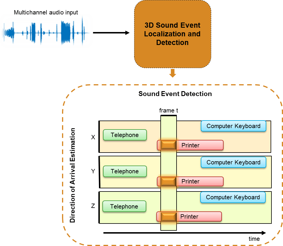
In this example, you train a deep learning model to perform sound localization and event detection from ambisonic data. The model consists of two independently trained convolutional recurrent neural networks (CRNN) [1]: one for sound event detection (SED), and one for direction of arrival (DOA) estimation. To explore the models trained in this example, see 3-D Sound Event Localization and Detection Using Trained Recurrent Convolutional Neural Network.
Introduction
Ambisonics is a popular 3-D sound format that has shown promise in tasks like sound source localization, speech enhancement, and source separation. Ambisonics is a full sphere surround sound format that contains a speaker-independent sound field representation (B-format). First order B-format ambisonic recordings contain components that correspond to the sound pressure captured by an omnidirectional microphone (W) and sound pressure gradients X, Y, and Z that correspond to front/back, left/right, and up/down captured by figure-of-eight capsules oriented along the three spatial axes. 3-D SELD has applications in virtual reality, robotics, smart homes, and defense.
You will train two separate models for the sound event detection task and the localization task. Both models are based on the convolutional recurrent neural network architecture described in [1]. The sound event detection task is formulated as a classification task. The sound event localization task estimates Cartesian coordinates of the sound source and is formulated as a regression task. You use the L3DAS21 data set [2] to train and validate the networks. To explore the models trained in this example, see 3-D Sound Event Localization and Detection Using Trained Recurrent Convolutional Neural Network.
Download and Prepare Data
This example uses a subset of the L3DAS21 Task 2 challenge data set [2]. The data set contains multiple-source and multiple-perspective (MSMP) B-format ambisonic audio recordings collected at a sampling rate of 32 kHz. The train and validation splits are provided with the data set. Each recording is one minute long and contains a simulated 3-D audio environment in which up to 3 simultaneous acoustic events may be active at the same time. In this example, you only use the data that contains non-overlapping sounds. The sound events belong to 14 sound classes. The labels are provided as csv files that contain the sound class, the Cartesian coordinates of the sound source, and the onset and offset time stamps.
Download the dataset.
downloadFolder = matlab.internal.examples.downloadSupportFile("audio","L3DAS21_ov1.zip");
dataFolder = tempdir;
unzip(downloadFolder,dataFolder)
dataset = fullfile(dataFolder,"L3DAS21_ov1");
Optionally Reduce Data Set
To train the networks with the entire data set and achieve a reasonable performance, set speedupExample to false. To run this example quickly, set speedupExample to true.
speedupExample =  false;
Create Datastores
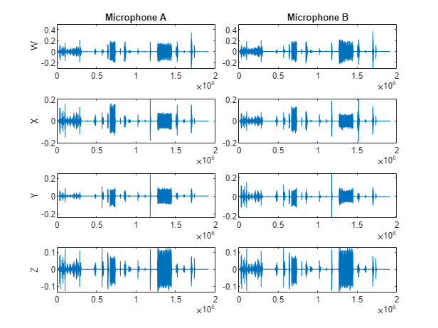
Create audioDatastore objects to ingest the data. Each data point in the data set consists of two B-format ambisonic recordings that correspond to the two microphones (A and B). For each data folder (train and validation), use subset to create two subsets corresponding to the two microphones.
adsTrain = audioDatastore(fullfile(dataset,"train","data"));
adsTrainA = subset(adsTrain,cellfun(@(c)endsWith(c,"A.wav"),adsTrain.Files));
adsTrainB = subset(adsTrain,cellfun(@(c)endsWith(c,"B.wav"),adsTrain.Files));

adsValidation = audioDatastore(fullfile(dataset,"validation","data"));
adsValidationA = subset(adsValidation,cellfun(@(c)endsWith(c,"A.wav"),adsValidation.Files));
adsValidationB = subset(adsValidation,cellfun(@(c)endsWith(c,"B.wav"),adsValidation.Files));
Reduce the data set if requested.
if speedupExample
    adsTrainA = subset(adsTrainA,1:2);
    adsTrainB = subset(adsTrainB,1:2);
end
Inspect Data
Preview the ambisonic recordings and plot the data.
micA = preview(adsTrainA);
micB = preview(adsTrainB);

tiledlayout(4,2,TileSpacing="tight")

nexttile
plot(micA(:,1))
title("Microphone A")
ylabel("W")

nexttile
plot(micB(:,1))
title("Microphone B")

nexttile
plot(micA(:,2))
ylabel("X")

nexttile
plot(micB(:,2))

nexttile
plot(micA(:,3))
ylabel("Y")

nexttile
plot(micB(:,3))

nexttile
plot(micB(:,4))
ylabel("Z")

nexttile
plot(micB(:,4))
Listen to a section of the data.
microphone =1; channel =
1; duration =
10; fs = 32e3; % Known sampling rate of data. s = [micA,micB]; data = s(1:round(duration*fs),channel + (microphone-1)*4); sound(data,fs)
Create Targets
Each data point in the data set has a corresponding CSV file containing the sound event class, the start and end times of the sound, and the location of the sound. Create a container to map between the sound classes and integers.
keySet = ["Chink_and_clink","Computer_keyboard","Cupboard_open_or_close","Drawer_open_or_close", ...
    "Female_speech_and_woman_speaking","Finger_snapping","Keys_jangling","Knock","Laughter", ...
    "Male_speech_and_man_speaking","Printer","Scissors","Telephone","Writing"];
valueSet = {1,2,3,4,5,6,7,8,9,10,11,12,13,14};
params.SoundClasses = containers.Map(keySet,valueSet);
Create a tabularTextDatastore to ingest the train file labels. Make sure the label files are in the same order as the data files. Preview a label file from the datastore.
[folder,fn] = fileparts(adsTrainA.Files);
targetPath = fullfile(strrep(folder,filesep+"data",filesep+"labels"),"label_" + strrep(fn,"_A","") + ".csv");
ttdsTrain = tabularTextDatastore(targetPath);

labelTable = preview(ttdsTrain)
labelTable=8×7 table
    0     0.5478     9.6651                             'Writing'     0.5000    -1.5000     0.3000
    0    11.5207    12.5342                     'Finger_snapping'     0.7500     1.2500         -1
    0    14.2552    16.0636                       'Keys_jangling'     0.5000    -1.5000     0.3000
    0    17.7278    18.8776                     'Chink_and_clink'     0.5000          1          0
    0    19.9502    20.4001                             'Printer'    -1.5000    -1.5000    -0.6000
    0    20.9939    23.4770              'Cupboard_open_or_close'    -0.5000     0.7500          0
    0    25.0318    25.7234                     'Chink_and_clink'         -2    -0.5000    -0.3000
    0    26.5471    27.4908    'Female_speech_and_woman_speaking'          1    -1.5000          0
The labels in the dataset are provided with time stamps in seconds. To create targets and train a network, you need to map the time stamps to frames. The total duration of each file is 60 seconds. You will divide each file into 600 frames for the target, meaning the model will make a prediction every 0.1 seconds.
params.Targets.TotalDuration = 60;
params.Targets.NumFrames = 600;
SED Targets
The supporting function, extractSEDTargets, uses the label data to create an SED target. The target is a one-hot encoded matrix of size numframes-by-numclasses. Frames with no sounds present are encoded as all-zero vectors.
SEDTargets = extractSEDTargets(labelTable,params);

[numframes,numclasses] = size(SEDTargets{1})
numframes = 600
numclasses =
14
Extract SED targets from the train and validation sets.
dsTTrain = transform(ttdsTrain,@(x)extractSEDTargets(x,params));
sedTTrain = readall(dsTTrain);

[folder,fn] = fileparts(adsValidationA.Files);
targetPath = fullfile(strrep(folder,filesep+"data",filesep+"labels"),"label_" + strrep(fn,"_A","") + ".csv");

ttdsValidation = tabularTextDatastore(targetPath);
dsTValidation = transform(ttdsValidation,@(x)extractSEDTargets(x,params));
sedTValidation = readall(dsTValidation);
DOA Targets
The supporting function, extractDOATargets, uses the label data to create a DOA target. The target is a matrix of size numframes-by-numaxis. The axis values correspond to the sound source location in 3-D space. Frames with no sounds present are encoded as all-zero vectors.
First, define a parameter to scale the target axis values so that they are between -1 and 1. This scaling is necessary because the DOA network you define later uses tanh activation as its final layer.
params.DOA.ScaleFactor = 2;
DOATargets = extractDOATargets(labelTable,params);

[numframes,numaxis] = size(DOATargets{1})
numframes = 600
numaxis =
3
Extract DOA targets from the train and validation sets.
dsTTrain = transform(ttdsTrain,@(x)extractDOATargets(x,params));
doaTTrain = readall(dsTTrain);

[folder,fn] = fileparts(adsValidationA.Files);
targetPath = fullfile(strrep(folder,filesep+"data",filesep+"labels"),"label_" + strrep(fn,"_A","") + ".csv");

ttdsValidation = tabularTextDatastore(targetPath);
dsTValidation = transform(ttdsValidation,@(x)extractDOATargets(x,params));
doaTValidation = readall(dsTValidation);
Sound Event Detection (SED)
Feature Extraction
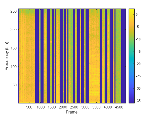
The sound event detection model uses log-magnitude short-time Fourier transforms (STFT) as predictors to the system. Specify a 512-point periodic Hamming window and a hop length of 400 samples.
params.SED.SampleRate = 32e3;
params.SED.HopLength = 400;
params.SED.Window = hamming(512,"periodic");
The supporting function, extractSTFT, takes a cell array of microphone readings and extracts the half-sided centered log-magnitude STFTs. The STFT features corresponding to both microphones are stacked along the third dimension.
stftFeats = extractSTFT({micA,micB},params);
[numfeaturesSED,numframesSED,numchannelsSED] = size(stftFeats)
numfeaturesSED = 256
numframesSED =
4800
numchannelsSED =
8
Plot the STFT features of one channel.
channel =7; figure imagesc(stftFeats(:,:,channel)) colorbar xlabel("Frame") ylabel("Frequency (bin)") set(gca,YDir="normal")
Extract features from the entire train and validation sets. First, combine the datastores corresponding to microphones A and B. Then, define a transform on the datastore so that reading from it returns the STFT. If you have Parallel Computing Toolbox™, you can speed up processing using the UseParallel flag of readall.
pFlag = ~isempty(ver("parallel")) && ~speedupExample;

trainDS = combine(adsTrainA,adsTrainB);
trainDS_T = transform(trainDS,@(x){extractSTFT(x,params)},IncludeInfo=false);
XTrain = readall(trainDS_T,UseParallel=pFlag);
valDS = combine(adsValidationA,adsValidationB);
valDS_T = transform(valDS,@(x){extractSTFT(x,params)},IncludeInfo=false);
XValidation = readall(valDS_T,UseParallel=pFlag);
Combine the predictor arrays with the previously computed SED target arrays.
trainSedDS = combine(arrayDatastore(XTrain,OutputType="same"),arrayDatastore(sedTTrain,OutputType="same"));
valSedDS = combine(arrayDatastore(XValidation,OutputType="same"),arrayDatastore(sedTValidation,OutputType="same"));
Training Options
Define training parameters for Adam optimization.
trainOptionsSED = struct( ...
    MaxEpochs=300, ...
    MiniBatchSize=4, ...
    InitialLearnRate=1e-5, ...
    GradientDecayFactor=0.01, ...
    SquaredGradientDecayFactor=0.0, ...
    ValidationPatience=25, ...
    LearnRateDropPeriod=100, ...
    LearnRateDropFactor=1);

if speedupExample
    trainOptionsSED.MaxEpochs = 1;
end
Create minibatchqueue (Deep Learning Toolbox) objects to read mini-batches from the train and validation datastores.
trainSEDmbq = minibatchqueue(trainSedDS, ...
    MiniBatchSize=trainOptionsSED.MiniBatchSize, ...
    OutputAsDlarray=[1,1], ...
    MiniBatchFormat=["SSCB","TCB"], ...
    OutputEnvironment=["auto","auto"]);

validationSEDmbq = minibatchqueue(valSedDS, ...
    MiniBatchSize=trainOptionsSED.MiniBatchSize, ...
    OutputAsDlarray=[1,1], ...
    MiniBatchFormat=["SSCB","TCB"], ...
    OutputEnvironment=["auto","auto"]);
Define Sound Event Detection (SED) Network
The network is implemented in two stages - Convolutional Neural Network (CNN) and Gated Recurrent Network (GRU). You will use a custom reshaping layer to recast the output of the CNN model into a sequence and pass that as the input to the RNN model. The custom reshaping layer is placed in your current folder when you open this example. The final output layer uses sigmoid activation.
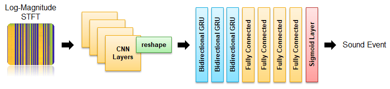
Define the CNN layers for the SED model.
seldnetCNNLayers = [
    imageInputLayer([numfeaturesSED,numframesSED,numchannelsSED],Normalization="none",Name="input")

    convolution2dLayer([3,3],64,Padding="same",Name="conv1")
    batchNormalizationLayer(Name="batchnorm1")
    reluLayer(Name="relu1")
    maxPooling2dLayer([8,2],Stride=[8,2],Padding="same",Name="maxpool1")

    convolution2dLayer([3,3],128,Padding="same",Name="conv2")
    batchNormalizationLayer(Name="batchnorm2")
    reluLayer(Name="relu2")
    maxPooling2dLayer([8,2],Stride=[8,2],Padding="same",Name="maxpool2")

    convolution2dLayer([3,3],256,Padding="same",Name="conv3")
    batchNormalizationLayer(Name="batchnorm3")
    reluLayer(Name="relu3")
    maxPooling2dLayer([2,2],Stride=[2,2],Padding="same",Name="maxpool3")

    convolution2dLayer([3,3],512,Padding="same",Name="conv4")
    batchNormalizationLayer(Name="batchnorm4")
    reluLayer(Name="relu4")
    maxPooling2dLayer([1,1],Stride=[1,1],Padding="same",Name="maxpool4")

    reshapeLayer("reshape")
    ];
netCNN = dlnetwork(seldnetCNNLayers);
Define the RNN layers for the SED model.
seldnetGRULayers = [
    sequenceInputLayer(1024,Name="sequenceInputLayer")

    bigruLayer(1024,256,Name="gru1")
    bigruLayer(512,256,Name="gru2")
    bigruLayer(512,256,Name="gru3")

    fullyConnectedLayer(1024,Name="fc1")
    reluLayer(Name="relu1")
    fullyConnectedLayer(1024,Name="fc2")
    reluLayer(Name="relu2")
    fullyConnectedLayer(1024,Name="fc3")
    reluLayer(Name="relu3")

    fullyConnectedLayer(params.SoundClasses.Count,Name="fc4")
    sigmoidLayer(Name="output")
    ];

netRNN = dlnetwork(seldnetGRULayers);
Create a struct to contain both the CNN and RNN sections of the full model.
sedModel.CNN = netCNN;
sedModel.RNN = netRNN;
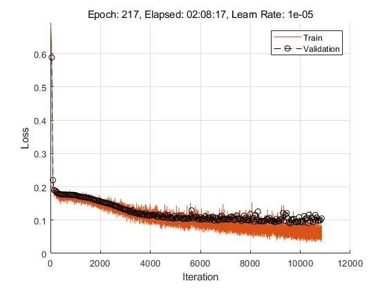
Train SED Network
Initialize variables to track the progress of the training.
iteration = 0;
averageGrad = [];
averageSqGrad = [];
epoch = 0;
bestLoss = Inf;
badEpochs = 0;
learnRate = trainOptionsSED.InitialLearnRate;
To display training progress, initialize the supporting object progresPlotterSELD. The supporting object, progressPlotterSELD, is placed in your current folder when you open this example.
pp = progressPlotterSELD();
Run the training loop.
rng(0)
while epoch < trainOptionsSED.MaxEpochs && badEpochs < trainOptionsSED.ValidationPatience

    epoch = epoch + 1;

    % Shuffle mini-batch queue.
    shuffle(trainSEDmbq)

    while hasdata(trainSEDmbq)

        % Update iteration counter.
        iteration = iteration + 1;

        % Read mini-batch of data.
        [X,T] = next(trainSEDmbq);

        % Evaluate the model gradients and loss using dlfeval and the modelLoss function.
        [loss,grad,state] = dlfeval(@modelLoss,sedModel,X,T);
        loss = loss/size(T,2);

        % Update state.
        sedModel.CNN.State = state.CNN;
        sedModel.RNN.State = state.RNN;

        % Update the network parameters using the Adam optimizer.
        [sedModel,averageGrad,averageSqGrad] = adamupdate(sedModel,grad,averageGrad, ...
            averageSqGrad,iteration,learnRate,trainOptionsSED.GradientDecayFactor,trainOptionsSED.SquaredGradientDecayFactor);

        % Update the training progress plot.
        updateTrainingProgress(pp,Epoch=epoch,LearnRate=learnRate,Iteration=iteration,Loss=loss);
    end

    % Perform validation after each epoch.
    loss = predictBatch(sedModel,validationSEDmbq);

    % Update the training progress plot with validation results.
    updateValidation(pp,Loss=loss,Iteration=iteration)

    % Create a checkpoint if the validation loss improved. If validation
    % loss did not improve, add to the number of bad epochs.
    if loss < bestLoss
        bestLoss = loss;
        badEpochs = 0;
        fileName = "SED-BestModel";
        save(fileName,"sedModel");
    else
        badEpochs = badEpochs + 1;
    end

    % Update learn rate
    if rem(epoch,trainOptionsSED.LearnRateDropPeriod)==0
        learnRate = learnRate*trainOptionsSED.LearnRateDropFactor;
    end

end
Direction of Arrival (DOA)
Feature Extraction
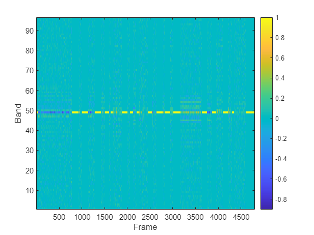
The direction of arrival estimation model uses generalized cross correlation phase transform (GCC-PHAT) as predictors to the system. Specify a 1024-point Hann window, a hop length of 400 samples, and the number of bands as 96.
params.DOA.SampleRate = 32e3;
params.DOA.Window = hann(1024);
params.DOA.NumBands = 96;
params.DOA.HopLength = 400;
Extract the GCC-PHAT features used as input predictors to the sound localization network. The GCC-PHAT algorithm measures the cross correlation between each pair of channels. The input signals have a total of 8 channels, so the output has a total of 28 measurements.
gccPhatFeats = extractGCCPHAT({micA,micB},params);
[numfeaturesDOA,timestepsDOA,numchannelsDOA] = size(gccPhatFeats)
numfeaturesDOA = 96
timestepsDOA =
4800
numchannelsDOA =
28
Plot the GCC-PHAT features of a channel pair.
channelpair =1; figure imagesc(gccPhatFeats(:,:,channelpair)) colorbar xlabel("Frame") ylabel("Band") set(gca,YDir="normal")
Extract features from the entire train and validation sets. If you have Parallel Computing Toolbox™, you can speed up processing using the UseParallel flag of readall.
pFlag = ~isempty(ver("parallel")) && ~speedupExample;

trainDS = combine(adsTrainA,adsTrainB);
trainDS_T = transform(trainDS,@(x){extractGCCPHAT(x,params)},IncludeInfo=false);
XTrain = readall(trainDS_T,UseParallel=pFlag);
Starting parallel pool (parpool) using the 'local' profile ... Connected to the parallel pool (number of workers: 6).
valDS = combine(adsValidationA,adsValidationB);
valDS_T = transform(valDS,@(x){extractGCCPHAT(x,params)},IncludeInfo=false);
XValidation = readall(valDS_T,UseParallel=pFlag);
Combine the predictor arrays with the previously compute DOA target arrays.
trainDOA = combine(arrayDatastore(XTrain,OutputType="same"),arrayDatastore(doaTTrain,OutputType="same"));
validationDOA = combine(arrayDatastore(XValidation,OutputType="same"),arrayDatastore(doaTValidation,OutputType="same"));
Training Options
Use the same train options you defined when training the SED network.
trainOptionsDOA = trainOptionsSED;
Create mini-batch queues for the train and validation sets.
trainDOAmbq = minibatchqueue(trainDOA, ...
    MiniBatchSize=trainOptionsDOA.MiniBatchSize, ...
    OutputAsDlarray=[1,1], ...
    MiniBatchFormat=["SSCB","TCB"], ...
    OutputEnvironment=["auto","auto"]);
validationDOAmbq = minibatchqueue(validationDOA, ...
    MiniBatchSize=trainOptionsDOA.MiniBatchSize, ...
    OutputAsDlarray=[1,1], ...
    MiniBatchFormat=["SSCB","TCB"], ...
    OutputEnvironment=["auto","auto"]);
Define Direction of Arrival (DOA) Network
The DOA network is very similar to the SED network defined earlier. The key differences are the size of the input layer and the final activation layer.
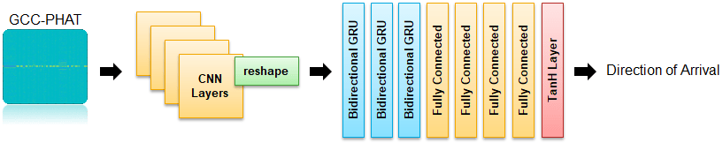
Update the SELDnet architecture used for the SED network for use with DOA estimation.
seldnetCNNLayers(1) = imageInputLayer([numfeaturesDOA,timestepsDOA,numchannelsDOA],Normalization="none",Name="input");
seldnetCNNLayers(5) = maxPooling2dLayer([3,2],Stride=[3,2],Padding="same",Name="maxpool1");
netCNN = dlnetwork(layerGraph(seldnetCNNLayers));

seldnetGRULayers(11) = fullyConnectedLayer(3,Name="fc4");
seldnetGRULayers(12) = tanhLayer(Name="output");
netRNN = dlnetwork(layerGraph(seldnetGRULayers));
Create a struct to contain both the CNN and RNN sections of the full model.
doaModel.CNN = netCNN;
doaModel.RNN = netRNN;
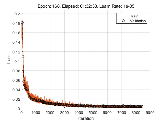
Train DOA Network
Initialize variables used in the training loop.
iteration = 0;
averageGrad = [];
averageSqGrad = [];
epoch = 0;
bestLoss = Inf;
badEpochs = 0;
learnRate = trainOptionsDOA.InitialLearnRate;
To display training progress, initialize the supporting object progressPlotterSELD. The supporting object, progressPlotterSELD, is placed in your current folder when you open this example.
pp = progressPlotterSELD();
Run the training loop.
rng(0)
while epoch < trainOptionsDOA.MaxEpochs && badEpochs < trainOptionsDOA.ValidationPatience

    epoch = epoch + 1;

    % Shuffle mini-batch queue.
    shuffle(trainDOAmbq)

    while hasdata(trainDOAmbq)

        % Update iteration counter.
        iteration = iteration + 1;

        % Read mini-batch of data.
        [X,T] = next(trainDOAmbq);

        % Evaluate the model gradients and loss using dlfeval and the modelLoss function.
        [loss,grad,state] = dlfeval(@modelLoss,doaModel,X,T);
        loss = loss/size(T,2);

        % Update state.
        doaModel.CNN.State = state.CNN;
        doModel.RNN.State = state.RNN;

        % Update the network parameters using the Adam optimizer.
        [doaModel,averageGrad,averageSqGrad] = adamupdate(doaModel,grad,averageGrad, ...
            averageSqGrad,iteration,learnRate,trainOptionsDOA.GradientDecayFactor,trainOptionsDOA.SquaredGradientDecayFactor);

        % Update the training progress plot
        updateTrainingProgress(pp,Epoch=epoch,LearnRate=learnRate,Iteration=iteration,Loss=loss);
    end

    % Perform validation after each epoch
    loss = predictBatch(doaModel,validationDOAmbq);

    % Update the training progress plot with validation results.
    updateValidation(pp,Loss=loss,Iteration=iteration)

    % Create a checkpoint if the validation loss improved. If validation
    % loss did not improve, add to the number of bad epochs.
    if loss < bestLoss
        bestLoss = loss;
        badEpochs = 0;
        fileName = "DOA-BestModel";
        save(fileName,"doaModel");
    else
        badEpochs = badEpochs + 1;
    end

    % Update learn rate
    if rem(epoch,trainOptionsDOA.LearnRateDropPeriod)==0
        learnRate = learnRate*trainOptionsDOA.LearnRateDropFactor;
    end
end
Evaluate System Performance
To evaluate your system's performance, use the location-sensitive detection error defined in [4]. Load the best-performing models.
sedModel = importdata("SED-BestModel.mat");
doaModel = importdata("DOA-BestModel.mat");
Location-sensitive detection is a joint metric that evaluates the results of both sound event detection and sound event localization tasks. In this type of evaluation, a true positive only occurs when the predicted label is correct, and the predicted location is within a predefined threshold of the true location. A threshold of 0.2 is used in this example which is about ~3% of the maximum possible error. To determine regions of silence in the prediction, set a confidence threshold on SED decisions. If the SED predictions are below that threshold, the frame is considered silence.
params.SpatialThreshold = 0.2;
params.SilenceThreshold = 0.1;
Compute the metrics for the validation data set using the computeMetrics supporting function.
results = computeMetrics(sedModel,doaModel,validationSEDmbq,validationDOAmbq,params);
results
results = struct with fields:
    precision: 0.4246
       recall: 0.4275
      f1Score: 0.4261
       avgErr: 0.1861
The computeMetrics supporting function can optionally smooth the decisions over time before evaluating the system. This option requires the Statistics and Machine Learning Toolbox™. Evaluate the system again, this time including the smoothing.
[results,cm] = computeMetrics(sedModel,doaModel,validationSEDmbq,validationDOAmbq,params,ApplySmoothing=true);
results
results = struct with fields:
    precision: 0.5077
       recall: 0.5084
      f1Score: 0.5080
       avgErr: 0.1659
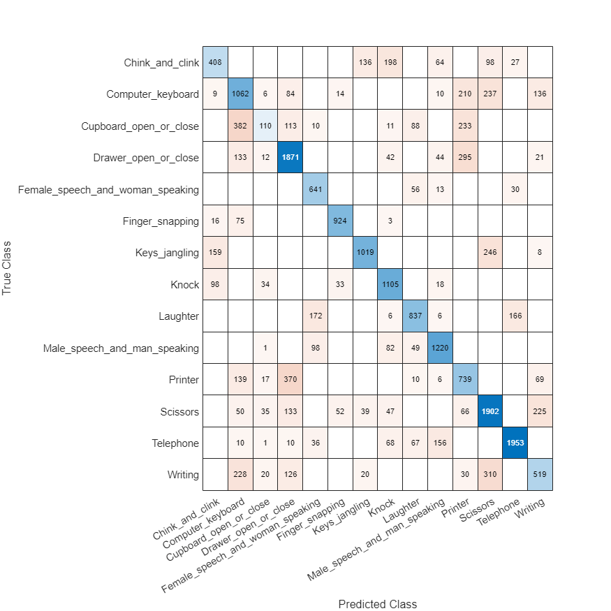
You can inspect the confusion matrix for SED predictions to get more insights on the prediction errors. The confusion matrix is only calculated over regions where there is an active sound source.
figure(Position=[100 100 800 800]);
confusionchart(cm,keys(params.SoundClasses))
Conclusion
For next steps, you can download and try out the pretrained models from this example in this second example showing inference: 3-D Sound Event Localization and Detection Using Trained Recurrent Convolutional Neural Network.
References
[1] Sharath Adavanne, Archontis Politis, Joonas Nikunen, and Tuomas Virtanen, "Sound event localization and detection of overlapping sources using convolutional recurrent neural networks," IEEE J. Sel. Top. Signal Process., vol. 13, no. 1, pp. 34–48, 2019.
[2] Eric Guizzo, Riccardo F. Gramaccioni, Saeid Jamili, Christian Marinoni, Edoardo Massaro, Claudia Medaglia, Giuseppe Nachira, Leonardo Nucciarelli, Ludovica Paglialunga, Marco Pennese, Sveva Pepe, Enrico Rocchi, Aurelio Uncini, and Danilo Comminiello "L3DAS21 Challenge: Machine Learning for 3D Audio Signal Processing," 2021.
[3] Yin Cao, Qiuqiang Kong, Turab Iqbal, Fengyan An, Wenwu Wang, and Mark D. Plumbley, "Polyphonic sound event detection and localization using a two-stage strategy," arXiv preprint: arXiv:1905.00268v4, 2019.
[4] Mesaros, Annamaria, Sharath Adavanne, Archontis Politis, Toni Heittola, and Tuomas Virtanen. "Joint Measurement of Localization and Detection of Sound Events." 2019 IEEE Workshop on Applications of Signal Processing to Audio and Acoustics (WASPAA), 2019. https://doi.org/10.1109/waspaa.2019.8937220.
Supporting Functions
Extract Direction of Arrival (DOA) Targets
function T = extractDOATargets(csvFile,params)
%EXTRACTDOATARGETS Extract direction of arrival (DOA) targets
% T = extractDOATargets(fileName,params) parses the CSV file
% fileName and returns a matrix, T. The target matrix is an N-by-3
% matrix, where N corresponds to the number of frames and 3 corresponds to
% the 3 axes describing location in 3-D space.

% Preallocate target matrix. A frame of all zeros corresponds to no sound
% source.
T = zeros(params.Targets.NumFrames,3);

% Quantize the time stamps for sound sources into frames.
startendTime = [csvFile.Start,csvFile.End];
startendFrame = time2frame(startendTime,params.Targets.TotalDuration,params.Targets.NumFrames);

% For each sound source, fill the target matrix sound source location for
% the appropriate number of frames.
for ii = 1:size(startendFrame,1)
    idx = startendFrame(ii,1):startendFrame(ii,2)-1;
    T(idx,:) = repmat([csvFile.X(ii),csvFile.Y(ii),csvFile.Z(ii)],numel(idx),1);
end

% Scale the target so that it is between -1 and 1 (the bounds of the tanh
% activation layer). Wrap the target in a cell array for convenient batch
% processing.
T = {T/params.DOA.ScaleFactor};
end
Extract Sound Event Detection (SED) Targets
function T = extractSEDTargets(csvFile,params)
%EXTRACTSEDTARGETS Extract sound event detection (SED) targets
% T = extractSEDTargets(fileName,params) parses the CSV file
% fileName and returns a matrix of SED targets, T. The target matrix is an N-by-K
% matrix, where N corresponds to the number of frames and K corresponds to
% the number of sound classes.

% Preallocate target matrix. A frame of all zeros corresponds to no sound
% source.
T = zeros(params.Targets.NumFrames,params.SoundClasses.Count);

% Quantize the time stamps for sound sources into frames.
startendTime = [csvFile.Start,csvFile.End];
startendFrame = time2frame(startendTime,params.Targets.TotalDuration,params.Targets.NumFrames);

% For each sound source, fill the appropriate column of the target matrix
% with a 1, indicating that the sound class is present in that frame.
for ii = 1:size(startendFrame,1)
    classID = params.SoundClasses(csvFile.Class{ii});
    T(startendFrame(ii,1):startendFrame(ii,2)-1,classID) = 1;
end

% Wrap the target in a cell array for convenient batch processing.
T = {T};
end
Short-Time Fourier Transform (STFT)
function X = extractSTFT(s,params)
%EXTRACTSTFT Extract log-magnitude of centered STFT
% X = extractSTFT({s1,s2},params) concatenates s1 and s2 and then
% extracts the one-sided log-magnitude STFT. The signals are padded before
% the STFT so that the first window is centered on the first sample. The
% output is trimmed to remove the 1st (DC) coefficient and the last
% spectrum. The input params defines the STFT.

% Concatenate the signals along the second (channel) dimension.
audio = cat(2,s{:});

% Extract the centered STFT.
N = numel(params.SED.Window);
overlapLength = N - params.SED.HopLength;
S = centeredSTFT(audio,params.SED.Window,overlapLength,N);

% Trim the 1st coefficient from all spectrums and trim the last spectrum.
S = S(2:end,1:end-1,:);

% Convert to log-magnitude. Use an offset to protect against log of zero.
mag = log(abs(S) + eps);

% Cast output to single precision.
X = single(mag);
end
Generalized Cross Correlation with Phase Transform (GCC-PHAT)
function X = extractGCCPHAT(s,params)
%EXTRACTGCCPHAT Extract generalized cross correlation phase transform (GCC-PHAT) features
% X = extractGCCPHAT({s1,s2},params) concatenates s1 and s2 and then
% extracts the GCC-PHAT for all pairs of channels.

% Concatenate the signals corresponding to the two microphones.
audio = cat(2,s{:});

% Count the total number of input channels.
nChan = size(audio,2);

% Calculate the total number of output channels.
numOutputChannels = nchoosek(nChan,2);

% Preallocate a NumFeatures-by-NumFrames-by-NumChannels feature (predictor)
% matrix.
numFrames = size(audio,1)/params.DOA.HopLength;
X = zeros(params.DOA.NumBands,numFrames,numOutputChannels);

% -----------------------------------
% Calculate GCC-PHAT for each pair of channels.
% Precompute STFT for each channel.
N = numel(params.DOA.Window);
overlapLength = N - params.DOA.HopLength;
micAB_stft = centeredSTFT(audio,params.DOA.Window,overlapLength,N);
conjmicAB_stft = conj(micAB_stft(:,:,2:end));
idx = 1;
for ii = 1:nChan - 1
    R = micAB_stft(:,:,ii).*conjmicAB_stft(:,:,ii:end);
    R = exp(1i .* angle(R));
    R = padarray(R, N/2 - 1,"post");
    gcc = fftshift(ifft(R,[],1,"symmetric"),1);
    X(:,:,idx:idx+size(R,3)-1) = gcc(floor(N/2+1 - (params.DOA.NumBands-1)/2):floor(N/2+1 + (params.DOA.NumBands-1)/2),1:end-1,:);

    idx = idx + size(R,3);
end
% -----------------------------------

% Cast output to single precision.
X = single(X);

end
Centered Short-Time Fourier Transform (STFT)
function s = centeredSTFT(audio,win,overlapLength,fftLength)
%CENTEREDSTFT Centered STFT
% s = centeredSTFT(audioIn,win,overlapLength,fftLength) computes an STFT
% with the first window centered around the first sample. The two ends are
% padded with the reflected audio signal.

% Pad front and back of input signal.
firstR = flip(audio(1:fftLength/2,:),1);
lastR = flip(audio(end - fftLength/2 + 1:end,:),1);
sig = cat(1,firstR,audio,lastR);

% Perform STFT.
s = stft(sig,Window=win,OverlapLength=overlapLength,FFTLength=fftLength,FrequencyRange="onesided");

end
Convert Time Stamp to Frame Number
function fnum = time2frame(t,dur,numFrames)
%TIME2FRAME Convert time stamp to frame number
% fnum = time2frame(t,dur,numFrames) maps the times t, which exist in dur,
% to a frame number if dur is divided into numFrames.

stp = dur/numFrames;

qt = round(t./stp).*stp;

fnum = floor(qt*(numFrames - 1)/dur) + 1;

end
Forward Pass Through CNN and RNN Networks
function [loss,cnnState,rnnState,Y3]  = forwardAll(model,X,T)
%FORWARDALL Forward pass of model through CNN and RNN networks
% [loss,cnnState,rnnState] = forwardAll(model,X,T) passes the predictors X
% through the model and returns the loss and the states of the networks in
% the model. The model is a struct containing a CNN network and an RNN
% network.
%
% [loss,cnnState,rnnState,Y] = forwardAll(model,X,T) also returns the final
% prediction of the model Y.

% Pass predictors through CNN.
[Y1,cnnState] = forward(model.CNN,X);

% Label the dimensions output from the CNN for consumption by the RNN.
Y2 = dlarray(Y1,"TCUB");

% Pass the predictors through the RNN.
[Y3,rnnState] = forward(model.RNN,Y2);

% Calculate the loss.
loss = seldNetLoss(Y3,T);

end
Full Model Prediction
function [loss,Y3]  = predictAll(model,X,T)
%PREDICTALL Model prediction through CNN and RNN networks
% [loss,prediction] = predictAll(model,X,T) passes the predictors X through
% the model and returns the loss and the model prediction. The model is a
% struct containing a CNN network and an RNN network.

% Pass predictors through CNN.
Y1 = predict(model.CNN,X);

% Label the dimensions output from the CNN for consumption by the RNN.
Y2 = dlarray(Y1,"TCUB");

% Pass the predictors through the RNN.
Y3 = predict(model.RNN,Y2);

% Calculate the loss.
loss = seldNetLoss(Y3,T);

end
Predict Batch
function loss = predictBatch(model,mbq)
%PREDICTBATCH Calculate the loss of mini-batch queue
% loss = predictBatch(model,mbq) returns the total loss calculated by
% passing the entire contents of the mini-batch queue through the model.

% Reset mini-batch queue and initialize counters.
reset(mbq)
loss = 0;
n = 0;

while hasdata(mbq)

    % Read the predictors and targets from mini-batch queue.
    [X,T] = next(mbq);

    % Pass the mini-batch through the model and calculate the loss.
    lss = predictAll(model,X,T);
    lss = lss/size(T,2);

    % Update the total loss.
    loss = loss + lss;

    % Sum number of datapoints.
    n = n + 1;

end

% Divide the total loss accumulated by the number of mini-batches.
loss = loss/n;

end
Compute Model Loss, Gradients, and Network States
function [loss,gradients,state] = modelLoss(model,X,T)
%MODELLOSS Compute model loss, gradients, and network states
% [loss,gradients,state] = modelLoss(model,X,T) passes the
% predictors X through the model and returns the loss, the gradients, and
% the states of the networks in the model. The model is a struct containing
% a CNN network and an RNN network.

% Pass the predictors through the model.
[loss,cnnState,rnnState] = forwardAll(model,X,T);

% Isolate the learnables.
allGrad.CNN = model.CNN.Learnables;
allGrad.RNN = model.RNN.Learnables;

state.CNN = cnnState;
state.RNN = rnnState;

% Calculate the gradients.
gradients = dlgradient(loss,allGrad);

end
Loss Function of SELDnet
function loss = seldNetLoss(Y,T)
%SELDNETLOSS Compute the SELDnet loss function for DOA or SED models
% loss = seldNetLoss(Y,T) returns the SELDnet loss given predictions Y and
% targets T. The loss function depends on the network (DOA or SED). The
% network is inferred by the dimensions of the target. For the DOA network,
% the loss function is mean-squared error. For the SED network, the loss
% function is crossentropy.

% Determine whether the targets correspond to the DOA network or SED
% network.
isDOAModel = size(T,find(dims(T)=='C'))==3;

if isDOAModel
    % Calculate MSE loss.
    doaLoss = mse(Y,T);
    doaLossFactor = 2 / (size(Y,1) * size(Y,3));
    loss = doaLoss * doaLossFactor; % To align with the original implementation
else
    % Calculate cross-entropy loss.
    loss = crossentropy(Y,T,ClassificationMode="multilabel",NormalizationFactor="all-elements");
end

loss = loss * size(T,2);

end
Compute Performance Metrics
function [r,cm] = computeMetrics(sedModel,doaModel,sedMBQ,doaMBQ,params,nvargs)
%COMPUTEMETRICS Compute performance metrics
% [r,cm] = computeMetrics(sedModel,doaModel,sedMBQ,doaMBW,params) returns
% a struct of performance metrics calculated over the SED and DOA
% validation mini-batch queues, and a confusion matrix cm valid SED
% regions.
arguments
    sedModel
    doaModel
    sedMBQ
    doaMBQ
    params
    nvargs.ApplySmoothing = false;
end

% Initialize counters.
TP = 0;
FP = 0;
FN = 0;
it = 0;
ct = 0;
err = 0;

sedYAll = [];
sedTAll = [];

% Loop over all the data.
reset(sedMBQ)
reset(doaMBQ)
while hasdata(sedMBQ)

    % Get the predictors, targets, and predictions for the SED model.
    [sedXb,sedTb] = next(sedMBQ);
    [~,sedYb]  = predictAll(sedModel,sedXb,sedTb);
    sedTb = extractdata(gather(sedTb));
    sedYb = extractdata(gather(sedYb));

    % Get the predictors, targets, and predictions for the DOA model.
    [doaXb,doaTb] = next(doaMBQ);
    [~,doaYb]  = predictAll(doaModel,doaXb,doaTb);
    doaTb = extractdata(gather(doaTb));
    doaYb = extractdata(gather(doaYb));
    doaYb = doaYb*params.DOA.ScaleFactor;
    doaTb = doaTb*params.DOA.ScaleFactor;

    % Loop over the mini-batches.
    for batch = 1:size(sedYb,2)

        % Isolate the predictors and targets for current data point.
        sedY = squeeze(sedYb(:,batch,:));
        sedT = squeeze(sedTb(:,batch,:));
        doaY = squeeze(doaYb(:,batch,:));
        doaT = squeeze(doaTb(:,batch,:));

        % If the SED predictions of a frame are all made with low
        % confidence (beneath a threshold), assume that there is no sound
        % source present.
        isActive = ~(sum(double(sedY<params.SilenceThreshold),1)==size(sedY,1));

        % Convert the SED predictors and targets from one-hot vectors to
        % scalars.
        [~,sedY] = max(sedY,[],1);
        sedY = sedY.*isActive;

        [isActive,sedT] = max(sedT,[],1);
        sedT = sedT.*isActive;

        % Smooth outputs.
        if nvargs.ApplySmoothing
            [doaY,sedY] = smoothOutputs(doaY,sedY,params);
        end

        % Perform location-sensitive detection.
        [tp,fp,fn,e,c] = locationSensitiveDetection(sedY,sedT,doaY,doaT,params);

        % Accumulate performance metrics.
        TP = TP + tp;
        FP = FP + fp;
        FN = FN + fn;
        err = err + e;
        ct = ct + c;

        sedYAll = [sedYAll sedY.*isActive]; %#ok<AGROW>
        sedTAll = [sedTAll sedT.*isActive]; %#ok<AGROW>
    end
    it = it + 1;
end

% Calculate performance metrics.
r.precision =  TP/(TP + FP + eps);
r.recall = TP / (TP + FN + eps);
r.f1Score = 2*(r.precision*r.recall)/(r.precision + r.recall + eps);
r.avgErr = err/ct;

% Calculate confusion matrix.
confmat = confusionmat(sedTAll,single(sedYAll),Order=0:14);
cm = confmat(2:end,2:end); % Remove the silence from the confusion matrix.
end
Location Sensitive Detection
function [TP,FP,FN,totErr,ct] = locationSensitiveDetection(sedY,sedT,doaY,doaT,params)
%LOCATIONSENSITIVEDETECTION Location sensitive detection
% [TP,FP,FN,totErr,ct] =
% locationSensitiveDetection(sedY,sedT,doaY,doaT,params) calculates the
% true positive, false positive, false negative, DOA total error, and
% number of active targets. The definitions of each metric are provided in
% [4].

% Calculate distance.
dist = vecnorm(doaY-doaT);

% Determine if sounds active for reference and predictions.
isReferenceActive = sedT~=0;
isPredictedActive = sedY~=0;

% Calculate the total DOA error for reference-active sections.
totErr = sum(dist.*isReferenceActive);

% Count total number of active targets.
ct = sum(isReferenceActive);

% Determine if the DOA is within threshold per frame.
isDOAnear = dist < params.SpatialThreshold;

% True positive:
TP = sum(isDOAnear & isReferenceActive & isPredictedActive & (sedT==sedY));

% False positive:
FP1 = sum(~isReferenceActive & isPredictedActive);
FP2 = sum(isReferenceActive & isPredictedActive & (sedT~=sedY | ~isDOAnear));
FP = FP1 + FP2;

% False negative:
FN1 = sum(isReferenceActive & ~isPredictedActive);
FN2 = sum(isReferenceActive & (sedT~=sedY | ~isDOAnear));
FN = FN1 + FN2;

end
Smooth Outputs
function [doaYSmooth,sedYSmooth] = smoothOutputs(doaY,sedY,params)
%SMOOTHOUTPUTS Smooth DOA and SED predictions over time
% [doaYSmooth,sedYSmooth] = smoothOutputs(doaY,sedY,params) smooths the DOA
% and SED predictions over time.

% Preallocate smoothed outputs.
doaYSmooth = doaY;
sedYSmooth = sedY;

% Cluster the DOA predictions.
clusters = clusterdata(doaY',Criterion="distance",Cutoff=params.SpatialThreshold);
stt = 1;
enn = 1;

while enn <= params.Targets.NumFrames

    if clusters(stt) == clusters(enn)
        enn = enn + 1;
    else
        doaYSmooth(:,stt:enn-1) = smoothDOA(doaY(:,stt:enn-1));
        sedYSmooth(:,stt:enn-1) = smoothSED(sedY(:,stt:enn-1));
        stt = enn;
    end

end

doaYSmooth(:,stt:enn-1) = smoothDOA(doaY(:,stt:enn-1));
sedYSmooth(:,stt:enn-1) = smoothSED(sedY(:,stt:enn-1));

sedYSmooth = round(movmedian(sedYSmooth,5));

end
Smooth DOA Prediction
function smoothed = smoothDOA(chunk)
%SMOOTHDOA Smooth DOA prediction
% smoothed = smoothDOA(chunk) smooths DOA predictions by replacing the
% values of each axis with the mean of that axis in the chunk. The mean is
% calculated after discarding the lower and upper quarters of data.

% Determine the length of the chunk, and then indices to cut out the middle
% half of the data.
chlen = size(chunk,2);
st = max(round(chlen*1/4),1);
en = max(round(chlen*3/4),1);

% Sort the spatial axes (columns).
dim = sort(chunk,2);

% Take the mean of the inner half.
smoothed = repmat(mean(dim(:,st:en),2),1,chlen);

end
Smooth SED Prediction
function smoothed = smoothSED(chunk)
%SMOOTHSED Smooth SED prediction
% smoothed = smoothSED(chunk) smooths SED predictions using the mode.

smoothed = repmat(mode(chunk),1,size(chunk,2));

end