このページの内容は最新ではありません。最新版の英語を参照するには、ここをクリックします。
raytrace
R2026aRF 伝播光線の表示または計算
説明
関数 raytrace は、引数 Map で定義された 3 次元モデルを使用してレイ トレーシング解析を実行し、伝播パスをプロットまたは計算します。関数は、送信機サイトから受信機サイトまでの受信電力 (dBm) またはパス損失 (dB) に応じて、各伝播パスを色分けします。
レイ トレーシング解析には表面反射とエッジ回折が含まれますが、コーナー回折、屈折、または拡散散乱の効果は含まれません。この関数は 100 MHz ~ 100 GHz の周波数をサポートします。この関数は、tx 入力に関連付けられた周波数の伝播パスを評価します。txsite オブジェクトの TransmitterFrequency プロパティを使用して、送信機サイトの動作周波数を指定します。レイ トレーシング解析の詳細については、無線通信のためのレイ トレーシングを参照してください。
raytrace( は、レイ トレーシング伝播モデル tx,rx,propmodel)propmodel を使用して伝播パスを検出します。レイ トレーシング伝播モデルを使用すると、反射と回折の最大数、パス損失のしきい値、建物と地形の材料などのプロパティを指定することができます。関数 propagationModel を使用して、レイ トレーシング伝播モデルを作成します。
raytrace(___, は、前の構文にある任意の入力の組み合わせに加えて、1 つ以上の名前と値の引数を使用してオプションを指定します。Name=Value)
rays = raytrace(___)rays の伝播パスを返します。
例
レイ トレーシング伝播モデルを使用して、シカゴでの反射伝播パスを表示します。
シカゴの建物を指定してサイト ビューアーを起動します。OpenStreetMap® ファイルの詳細については、[1] を参照してください。
viewer = siteviewer(Buildings="chicago.osm");2 つの異なる建物の近くに送信機サイトと受信機サイトを作成します。
tx = txsite(Latitude=41.8800, ...
    Longitude=-87.6295, ...
    TransmitterFrequency=2.5e9);
show(tx)
rx = rxsite(Latitude=41.8813452, ...
    Longitude=-87.629771, ...
    AntennaHeight=30);
show(rx)
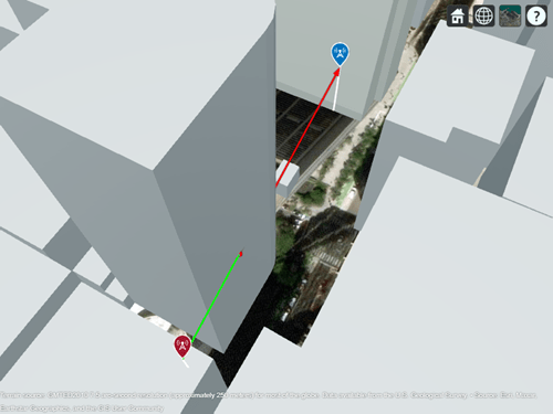
見通し内パス上の障害物を表示します。
los(tx,rx)
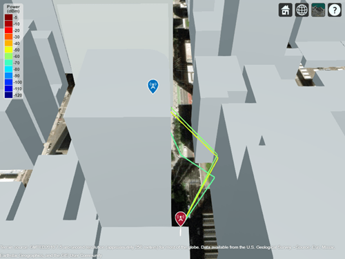
反射を伴う伝播パスを表示します。既定では、関数 raytrace は SBR 法を使用し、最大 2 回の反射を伴う伝播パスを計算します。
raytrace(tx,rx)
付録
[1] OpenStreetMap ファイルは、クラウドソーシングによる世界中の地図データへのアクセスを提供する https://www.openstreetmap.org からダウンロードされたものです。このデータは Open Data Commons Open Database License (ODbL) https://opendatacommons.org/licenses/odbl/ によりライセンスされています。
シカゴの建物を指定してサイト ビューアーを起動します。OpenStreetMap® ファイルの詳細については、[1] を参照してください。
viewer = siteviewer(Buildings="chicago.osm");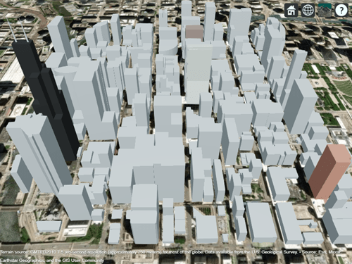
建物の上に送信機サイトを作成します。
tx = txsite(Latitude=41.8800, ...
    Longitude=-87.6295, ...
    TransmitterFrequency=2.5e9);
別の建物の近くに受信機サイトを作成します。
rx = rxsite(Latitude=41.881352, ...
    Longitude=-87.629771, ...
    AntennaHeight=30);
レイ トレーシング伝播モデルを作成します。MATLAB® は、RayTracing オブジェクトを使用してこのモデルを表現します。既定では、伝播モデルは SBR 法を使用し、最大 2 回の表面反射を伴う伝播パスを検出します。
pm = propagationModel("raytracing");受信機サイト、送信機サイト、および伝播モデルを使用して信号強度を計算します。
ssTwoReflections = sigstrength(rx,tx,pm)
ssTwoReflections =
-54.3151
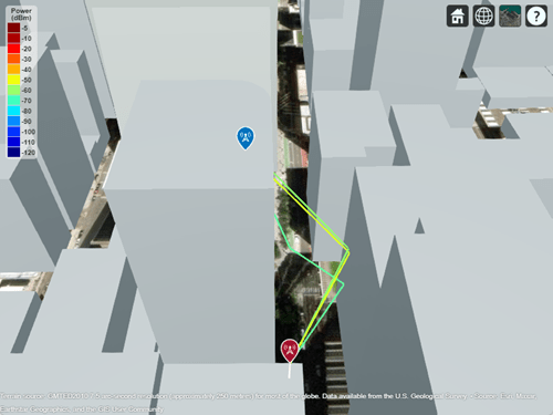
伝播パスをプロットします。
raytrace(tx,rx,pm)
RayTracing オブジェクトを変更して、最大 5 回の反射を伴うパスを検出します。次に、信号強度を再計算します。
pm.MaxNumReflections = 5;
ssFiveReflections = sigstrength(rx,tx,pm)
ssFiveReflections =
-53.3965
RayTracing オブジェクトは、既定で、地形の材料としてコンクリートを使用し、建物の材料として OpenStreetMap ファイルから取得した材料を使用します。OpenStreetMap ファイルで材料が指定されていない場合、モデルはコンクリートを使用します。建物と地形の材料タイプを変更して、完全な電気伝導体をモデル化します。
pm.TerrainMaterial = "PEC";
pm.BuildingsMaterial = "PEC";

ssPerfect = sigstrength(rx,tx,pm)
ssPerfect =
-38.9334
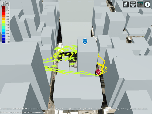
更新された伝播モデルの伝播パスをプロットします。
raytrace(tx,rx,pm)
付録
[1] OpenStreetMap ファイルは、クラウドソーシングによる世界中の地図データへのアクセスを提供する https://www.openstreetmap.org からダウンロードされたものです。このデータは Open Data Commons Open Database License (ODbL) https://opendatacommons.org/licenses/odbl/ によりライセンスされています。
香港の建物を指定してサイト ビューアーを起動します。OpenStreetMap® ファイルの詳細については、[1] を参照してください。
viewer = siteviewer(Buildings="hongkong.osm");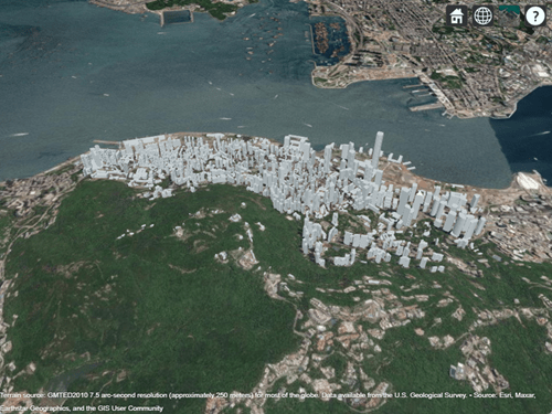
密集した都市環境の小さいセル シナリオをモデル化する送信機サイトと受信機サイトを作成します。
tx = txsite(Name="Small cell transmitter", ...
    Latitude=22.2789, ...
    Longitude=114.1625, ...
    AntennaHeight=10, ...
    TransmitterPower=5, ...
    TransmitterFrequency=28e9);
rx = rxsite(Name="Small cell receiver", ...
    Latitude=22.2799, ...
    Longitude=114.1617, ...
    AntennaHeight=1);
レイ トレーシング伝播モデルを作成します。MATLAB は、RayTracing オブジェクトを使用してこのモデルを表現します。発射された光線間で低い平均角度を使用し、最大 5 つのパス反射を伴うパスを検出し、完全な電気伝導体をモデル化する建物と地形の材料タイプを使用するようにモデルを構成します。既定では、モデルは SBR 法を使用します。
pm = propagationModel("raytracing", ...
    MaxNumReflections=5, ...
    AngularSeparation="low", ...
    BuildingsMaterial="PEC", ...
    TerrainMaterial="PEC");
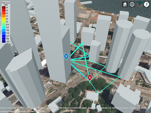
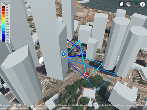
伝播パスを可視化し、対応するパス損失を計算します。
raytrace(tx,rx,pm,Type="pathloss")
raysPerfect = raytrace(tx,rx,pm,Type="pathloss");
plPerfect = [raysPerfect{1}.PathLoss]
plPerfect = 1×13

  104.2656  103.5699  112.0092  109.3137  111.2840  111.9979  112.4416  108.1505  111.2825  111.3905  117.7506  116.5906  117.7638
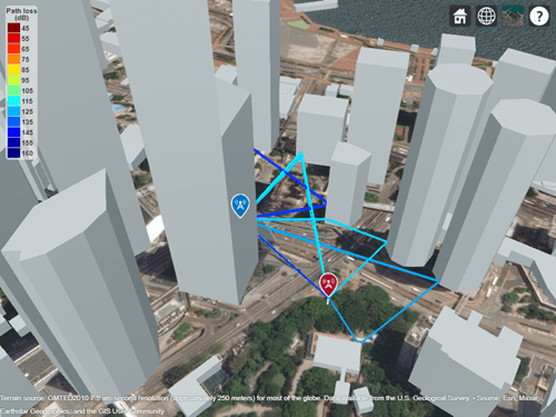
建物と地形の材料タイプをそれぞれガラスとコンクリートに設定します。次に、伝播パスを再び可視化し、対応するパス損失を再計算します。既定では、モデルは最も強いパスより 40 デシベルを超えて弱いパスを破棄するため、モデルは 1 つ少ないパスを検出します。最初のパス損失値は、見通し内伝播パスに対応しているため、変わっていません。
pm.BuildingsMaterial = "glass";
pm.TerrainMaterial = "concrete";

raytrace(tx,rx,pm,Type="pathloss")
raysMtrls = raytrace(tx,rx,pm,Type="pathloss");
plMtrls = [raysMtrls{1}.PathLoss]
plMtrls = 1×12

  104.2656  106.1249  119.2135  121.2269  122.3753  121.5228  126.8929  124.1284  122.7842  127.4910  138.9922  140.4998
雨と気体の伝播モデルをレイ トレーシング モデルに追加して、大気損失を組み込みます。次に、伝播パスを再び可視化し、対応するパス損失を再計算します。
pm = pm + propagationModel("rain") + propagationModel("gas");

raytrace(tx,rx,pm,Type="pathloss")
raysAtmospheric = raytrace(tx,rx,pm,Type="pathloss");
plAtmospheric = [raysAtmospheric{1}.PathLoss]
plAtmospheric = 1×11

  105.3233  107.1836  121.7958  123.1202  124.9592  124.1122  129.6076  126.0225  125.3745  130.2060  143.9945
付録
[1] OpenStreetMap ファイルは、クラウドソーシングによる世界中の地図データへのアクセスを提供する https://www.openstreetmap.org からダウンロードされたものです。このデータは Open Data Commons Open Database License (ODbL) https://opendatacommons.org/licenses/odbl/ によりライセンスされています。
この例では、以下の方法を説明します。
モデルがメートルの単位を使用するための STL ファイルのスケーリング。
サイト ビューアーでのスケーリング モデルの表示。
レイ トレーシングを使用した、送信機から受信機までの伝播パスの計算と表示。
直交 txsite オブジェクトおよび直交 rxsite オブジェクトはメートル単位の位置座標を必要としますが、STL ファイルでは他の単位を使用することができます。STL ファイルがメートルを使用していない場合は、サイト ビューアーにインポートする前にモデルをスケーリングしなければなりません。
STL ファイルをインポートして表示します。このファイルはテーブル 1 台と椅子が 4 脚ある小さい会議室をモデル化したものです。名前と値の引数 SceneModelScale を指定して、モデルをスケーリングします。この例では、STL 単位からメートルへの変換係数が 0.9 であると仮定しています。
viewer = siteviewer(SceneModel="conferenceroom.stl",SceneModelScale=0.9);
R2023b より前: 関数 stlread を使用してモデルを triangulation オブジェクトに読み取り、座標をスケーリングして新しい triangulation オブジェクトを作成してから、新しい triangulation オブジェクトをサイト ビューアーに読み取ります。
送信機サイトを壁の近くに、受信機サイトをテーブルの下に作成して表示します。直交座標を使用してメートル単位で位置を指定します。
tx = txsite("cartesian", ...
    AntennaPosition=[-1.25; -1.25; 1.9], ...
    TransmitterFrequency=2.8e9);
show(tx,ShowAntennaHeight=false)

rx = rxsite("cartesian", ...
    AntennaPosition=[0.3; 0.2; 0.5]);
show(rx,ShowAntennaHeight=false)
パンするには左クリックします。ズームするには右クリックまたはスクロール ホイールを使用します。表示を回転させるには、中央ボタンをクリックしてドラッグするか、"Ctrl" を押しながら左クリックしてドラッグします。

直交座標のレイ トレーシング伝播モデルを作成します。これは、MATLAB が RayTracing オブジェクトを使用して表現します。最大 1 回の反射と 1 回の回折を伴う光線を計算します。表面材料を木に設定します。既定では、モデルは SBR 法を使用します。
pm = propagationModel("raytracing", ...
    CoordinateSystem="cartesian", ....
    MaxNumReflections=1, ...
    MaxNumDiffractions=1, ...
    SurfaceMaterial="wood");
伝播パスを計算し、結果を comm.Ray オブジェクトの cell 配列として返します。光線を抽出してプロットします。
r = raytrace(tx,rx,pm);
r = r{1};
plot(r)
光線をクリックして、光線に関する情報を表示します。

R2023b 以降
RoadRunner を使用して作成された glTF™ ファイルから 3 次元モデルを表示します。RoadRunner は、自動運転システムをシミュレートおよびテストするための 3 次元シーンを設計できる対話型エディターです。
サンプルの glTF ファイルを保存するための一時フォルダーを作成します。downloadGLTFFile 補助関数を使用し、ファイルをフォルダーにダウンロードします。この補助関数は、この例にサポート ファイルとして添付されています。
dataDir = fullfile(tempdir,"IntersectionAndBuildings");
if ~exist(dataDir,"dir")
    mkdir(dataDir)
end
downloadGLTFFile(dataDir)
バイナリ ファイルの名前を指定します。次に、サイト ビューアーを使用し、glTF ファイルをインポートして表示します。サイト ビューアーは、ファイルに保存されている色とテクスチャを使用してモデルを表示します。
filename = fullfile(dataDir,"IntersectionAndBuildings.glb");
viewer = siteviewer(SceneModel=filename,ShowEdges=false,ShowOrigin=false);
カメラの位置とカメラの回転角度を変更してビューを調整します。位置はメートル、回転角度は度を使用して指定します。
campos(viewer,-26,-57,37)
campitch(viewer,-25)
camheading(viewer,-26)
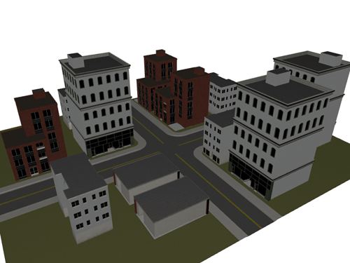
サイト ビューアーは、ファイルに保存されている各材料名を、サポートされている材料名と照合することで、シーン内の表面に材料を割り当てます。材料および照合で一致した材料のサブセットを表示します。既定では、レイ トレーシング解析関数は変数 MatchedCatalogMaterial に格納されている材料を使用します。
viewer.Materials(1:5,:)
ans=5×2 table
       Material       MatchedCatalogMaterial
    ______________    ______________________

    "Metal_Trim"            "metal"
    "Glass"                 "glass"
    "Stone_Trim"            "marble"
    "Roof_Asphalt"          "concrete"
    "Bricks_Red"            "brick"
建物の上に送信機サイトを作成し、建物群の後ろに受信機サイトを作成します。直交座標を使用してメートル単位で位置を指定します。
tx = txsite("cartesian",AntennaPosition=[18;38;22]);
rx = rxsite("cartesian",AntennaPosition=[-40;-35;1]);
直交座標のレイ トレーシング伝播モデルを作成します。これは、MATLAB® が RayTracing オブジェクトを使用して表現します。最大 2 回の反射 (既定) と 1 回の回折を伴う伝播パスを検出するようにモデルを構成します。
pm = propagationModel("raytracing", ...
    CoordinateSystem="cartesian", ...
    MaxNumDiffractions=1);
伝播パスを計算し、結果を comm.Ray オブジェクトの cell 配列として返します。cell 配列から伝播パスを抽出します。
rays = raytrace(tx,rx,pm);
rays = rays{1};
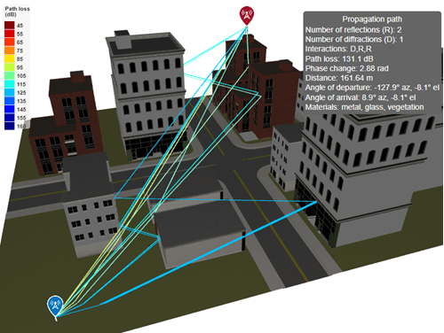
送信機サイト、受信機サイト、および伝播パスを表示します。カメラの位置とカメラの回転角度を変更してビューを調整します。
show(tx)
show(rx)
plot(rays)

campos(viewer,-22,-78,61)
campitch(viewer,-37)
camheading(viewer,-13)
パスをクリックして、パスに関する情報を表示します。相互作用する材料が情報ボックスに表示されます。
入力引数
名前と値の引数
オプションの引数のペアを Name1=Value1,...,NameN=ValueN として指定します。ここで、Name は引数名で、Value は対応する値です。名前と値の引数は他の引数の後に指定しなければなりませんが、ペアの順序は重要ではありません。
例: raytrace(tx,rx,Type="pathloss") は、パス損失に基づいてパスを色分けします。
R2021a より前では、コンマを使用して名前と値をそれぞれ区切り、Name を引用符で囲みます。
例: raytrace(tx,rx,"Type","pathloss") は、パス損失に基づいてパスを色分けします。
プロットする量のタイプ。次のオプションのいずれかとして指定します。
"power"— dBm 単位の受信電力に基づいてパスを色分けします。受信電力を計算するレイ トレーシング モデルの詳細については、無線通信のためのレイ トレーシングのPower at Receiverのセクションを参照してください。"pathloss"— dB 単位のパス損失に基づいてパスを色分けします。
データ型: char | string
伝播モデル。次のオプションのいずれかとして指定します。
"raytracing"— SBR 法を使用し、最大 2 回の反射と 0 回の回折を伴うパスを検出し、最も強いパスより 40 dB を超えて弱いパスを破棄します。RayTracingオブジェクト — レイ トレーシング伝播モデル。関数propagationModelを使用してRayTracingオブジェクトを作成します。RayTracingオブジェクトを使用すると、レイ トレーシング手法、反射と回折の最大数、パス損失のしきい値、建物と地形の材料などのプロパティを指定することができます。レイ トレーシング手法の違いの詳細については、伝播モデルの選択を参照してください。CompositePropagationModelオブジェクト — 合成伝播モデル。このモデルには、レイ トレーシング伝播モデルを組み込まなければなりません。add関数を使用して、個別の伝播モデルから合成伝播モデルを作成します。組み合わせることができる伝搬モデルのタイプの詳細については、伝播モデルの選択を参照してください。
propmodel 引数を使用して伝播モデルを指定することもできます。propmodel と PropagationModel の両方を指定した場合、関数は PropagationModel の値を使用します。
データ型: char | string
カラーマップの色の範囲。[min max] の形式の 2 要素の数値行ベクトルとして指定します。
単位と既定値は Type の値によって異なります。
"power"– 単位は dBm で、既定値は[-120 -5]です。"pathloss"– 単位は dB で、既定値は[45 160]です。
色の範囲は、カラーマップの最初と最後の色にマッピングされる値を示します。この関数は、色の範囲の最小値より小さい値の伝播パスをプロットしません。
データ型: double
伝播パスのカラーマップ。カラーマップ名として指定するか、M 個の個別の色を定義する RGB 3 成分から成る M 行 3 列の配列として指定します。
次の表はカラーマップ名の一覧です。
| カラーマップ名 | カラー スケール |
|---|---|
|
|
|
|
|
|
|
|
|
|
|
|
|
|
|
|
|
|
|
|
|
|
|
|
|
|
|
|
|
|
|
|
|
|
|
|
|
|
|
|
|
|
|
|






















データ型: char | string | double
サイト ビューアーでの色の凡例の表示。数値または logical の 1 (true) または 0 (false) として指定します。
可視化または表面データのマップ。siteviewer オブジェクト、triangulation オブジェクト、string スカラー、文字ベクトルのいずれかとして指定します。有効な既定値は、座標系に応じて異なります。
| 座標系 | 有効なマップ値 | 既定のマップ値 |
|---|---|---|
"geographic" |
|
|
"cartesian" |
|
|
a Alignment of boundaries and region labels are a presentation of the feature provided by the data vendors and do not imply endorsement by MathWorks®. | ||
ほとんどの場合、この引数を siteviewer や "none" 以外の値として指定した場合は出力引数も指定しなければなりません。
出力引数
ヒント
raytrace 関数によって作成される comm.Ray オブジェクトは、入力である txsite オブジェクトおよび rxsite オブジェクトの Antenna プロパティに格納されたアンテナ アレイのパターンを使用してパス損失を計算します。既定では、raytrace 関数は、最も強い伝播パスより 40 dB を超えて弱い伝播パスを破棄します。その結果、アンテナが偏波している場合、raytrace 関数は一部の comm.Ray オブジェクトを予期せず破棄することがあります。txsite オブジェクトおよび rxsite オブジェクトの Antenna プロパティを "isotropic" に設定することで、追加の伝播パスを調査できます。または、RayTracing 伝播モデル オブジェクトを作成し、RayTracing オブジェクトの MaxRelativePathLoss プロパティを Inf に設定して、RayTracing オブジェクトを raytrace 関数への入力として指定します。
参照
[1] International Telecommunications Union Radiocommunication Sector. Effects of Building Materials and Structures on Radiowave Propagation Above About 100MHz. Recommendation P.2040. ITU-R, approved August 23, 2023. https://www.itu.int/rec/R-REC-P.2040/en.
[2] International Telecommunications Union Radiocommunication Sector. Electrical Characteristics of the Surface of the Earth. Recommendation P.527. ITU-R, approved September 27, 2021. https://www.itu.int/rec/R-REC-P.527/en.
[3] Mohr, Peter J., Eite Tiesinga, David B. Newell, and Barry N. Taylor. “Codata Internationally Recommended 2022 Values of the Fundamental Physical Constants.” NIST, May 8, 2024. https://www.nist.gov/publications/codata-internationally-recommended-2022-values-fundamental-physical-constants.
[4] "IEEE Standard Definitions of Terms for Antennas." IEEE Std 145-2013 (Revision of IEEE Std 145-1993), March 2014, 1–50. https://doi.org/10.1109/IEEESTD.2014.6758443.
拡張機能
バージョン履歴
R2019b で導入SBR 法を使用して伝播パスを検出する際、MATLAB は、単精度浮動小数点の計算を使用して、各パスの幾何学的精度が正確になるように結果を修正します。以前のリリースでは、パスの幾何学的精度が近似的でした。
たとえば、次のコードは、既定の SBR 法を使用して送信機と受信機の間の伝播パスを検出し、そのパスを comm.Ray オブジェクトとして返します。R2022b では、関数 raytrace は 7 つの伝播パスを検出します。以前のリリースでは、関数は 8 つの伝播パスを概算し、そのうちの 1 つが重複パスになります。
viewer = siteviewer(Buildings="hongkong.osm");

tx = txsite(Latitude=22.2789,Longitude=114.1625,AntennaHeight=10, ...
   TransmitterPower=5,TransmitterFrequency=28e9);
rx = rxsite(Latitude=22.2799,Longitude=114.1617,AntennaHeight=1);

rSBR = raytrace(tx,rx)
raytrace(tx,rx)
| R2022b | R2022a |
|---|---|
rSBR =

  1×1 cell array

    {1×7 comm.Ray}
| rSBR =
1×1 cell array
{1×8 comm.Ray}
|


R2022b で SBR 法を使用して計算されたパスは、イメージ手法を使用して計算されたパスとより密接に一致します。イメージ手法は、正確な幾何学的精度ですべての可能なパスを検出します。たとえば、次のコードはイメージ手法を使用して、同じ送信機と受信機の間の伝播パスを検出します。
viewer = siteviewer(Buildings="hongkong.osm");

tx = txsite(Latitude=22.2789,Longitude=114.1625, ...
   AntennaHeight=10,TransmitterPower=5, ...
   TransmitterFrequency=28e9);
rx = rxsite(Latitude=22.2799,Longitude=114.1617, ...
   AntennaHeight=1);

pm = propagationModel("raytracing",Method="image",MaxNumReflections=2);

rImage = raytrace(tx,rx,pm)
rImage =

  1×1 cell array

    {1×7 comm.Ray}
この場合、SBR 法はイメージ手法と同じ数の伝播パスを検出します。一般に、SBR 法では、イメージ手法によって検出されるパスのサブセットを検出します。イメージ手法と SBR 法の両方で同じパスが検出される場合、そのパスに沿った点は、単精度浮動小数点値のマシン精度の許容誤差内で同じになります。
次のコードは、SBR 法とイメージ手法によって計算されたパス損失を 0.0001 の許容誤差内で比較します。
abs([rSBR{1}.PathLoss]-[rImage{1}.PathLoss]) < 0.0001ans = 1×7 logical array 1 1 1 1 1 1 1
パス損失は、指定された許容誤差内で同じです。
その結果、関数 raytrace は、R2022b では以前のリリースとは異なる結果を返す可能性があります。
この関数は、無効なパスまたは重複するパスを破棄するため、異なる数の
comm.Rayオブジェクトを返すことがあります。この関数は、おおよそのパスではなく正確なパスを計算するため、異なる
comm.Rayオブジェクトを返すことがあります。

