このページは機械翻訳を使用して翻訳されました。最新版の英語を参照するには、ここをクリックします。
GroundTrack
シナリオ内の衛星またはプラットフォームに属する地上追跡オブジェクト
説明
GroundTrack は、シナリオ内の衛星またはプラットフォームに属する地上トラック オブジェクトを定義します。
作成
Satellite または Platform (Satellite Communications Toolbox) オブジェクトの groundTrack オブジェクト関数を使用して GroundTrack オブジェクトを作成できます。
プロパティ
衛星シナリオ ビューアーで視覚化される地上トラックの周期。'LeadTime' と秒単位の正のスカラーとして指定します。
既定値は次のとおりです。
衛星シナリオ
StartTimeからStopTimeまで(OrbitPropagatorが'ephemeris'に設定されている場合)軌道が放物線または双曲線で、
OrbitPropagatorが'numerical'に設定されている場合の衛星シナリオStartTimeからStopTimeそれ以外の場合は 1 軌道周期です。
Viewer で視覚化される地上軌跡履歴の期間。'TrailTime' と秒単位の正のスカラーで指定します。
既定値は次のとおりです。
衛星シナリオ
StartTimeからStopTimeまで(OrbitPropagatorが'ephemeris'に設定されている場合)軌道が放物線または双曲線で、
OrbitPropagatorが'numerical'に設定されている場合の衛星シナリオStartTimeからStopTimeそれ以外の場合は 1 軌道周期です。
地上トラックの視覚的な幅(ピクセル単位)。'LineWidth' と (0 10] の範囲のスカラーで指定します。
ライン幅をピクセルの幅より細くすることはできません。システムでライン幅をピクセルの幅より細い値に設定すると、ラインは 1 ピクセル幅で表示されます。
将来の地上トラック ラインの色。'LeadLineColor' と RGB トリプレット、16 進カラー コード、色名、または短縮名として指定します。
カスタム色を使用する場合は、RGB 3 成分または 16 進数カラー コードを指定します。
RGB 3 成分は、色の赤、緑、青成分の強度を指定する 3 成分の行ベクトルです。強度値は
[0,1]の範囲でなければなりません。たとえば[0.4 0.6 0.7]のようになります。16 進数カラー コードは、ハッシュ記号 (
#) で始まり、3 桁または 6 桁の0からFまでの範囲の 16 進数が続く string スカラーまたは文字ベクトルです。この値は大文字と小文字を区別しません。したがって、カラー コード"#FF8800"、"#ff8800"、"#F80"、および"#f80"は等価です。
あるいは、名前を使用して一部の一般的な色を指定できます。次の表に、名前の付いた色オプション、等価の RGB 3 成分、および 16 進数カラー コードを示します。
| 色名 | 省略名 | RGB 3 成分 | 16 進数カラー コード | 外観 |
|---|---|---|---|---|
"red" | "r" | [1 0 0] | "#FF0000" |
|
"green" | "g" | [0 1 0] | "#00FF00" |
|
"blue" | "b" | [0 0 1] | "#0000FF" |
|
"cyan" | "c" | [0 1 1] | "#00FFFF" |
|
"magenta" | "m" | [1 0 1] | "#FF00FF" |
|
"yellow" | "y" | [1 1 0] | "#FFFF00" |
|
"black" | "k" | [0 0 0] | "#000000" |
|
"white" | "w" | [1 1 1] | "#FFFFFF" |
|


MATLAB® の多くのタイプのプロットで使用されている既定の色の RGB 3 成分および 16 進数カラー コードを次に示します。
| RGB 3 成分 | 16 進数カラー コード | 外観 |
|---|---|---|
[0 0.4470 0.7410] | "#0072BD" |
|
[0.8500 0.3250 0.0980] | "#D95319" |
|
[0.9290 0.6940 0.1250] | "#EDB120" |
|
[0.4940 0.1840 0.5560] | "#7E2F8E" |
|
[0.4660 0.6740 0.1880] | "#77AC30" |
|
[0.3010 0.7450 0.9330] | "#4DBEEE" |
|
[0.6350 0.0780 0.1840] | "#A2142F" |
|
![Sample of RGB triplet [0 0.4470 0.7410], which appears as dark blue](colororder1.png)
![Sample of RGB triplet [0.8500 0.3250 0.0980], which appears as dark orange](colororder2.png)
![Sample of RGB triplet [0.9290 0.6940 0.1250], which appears as dark yellow](colororder3.png)
![Sample of RGB triplet [0.4940 0.1840 0.5560], which appears as dark purple](colororder4.png)
![Sample of RGB triplet [0.4660 0.6740 0.1880], which appears as medium green](colororder5.png)
![Sample of RGB triplet [0.3010 0.7450 0.9330], which appears as light blue](colororder6.png)
![Sample of RGB triplet [0.6350 0.0780 0.1840], which appears as dark red](colororder7.png)
例: 'blue'
例: [0 0 1]
例: '#0000FF'
地上トラックライン履歴の色。'TrailLineColor' と RGB トリプレット、16 進カラー コード、色名、または短縮名として指定します。
カスタム色を使用する場合は、RGB 3 成分または 16 進数カラー コードを指定します。
RGB 3 成分は、色の赤、緑、青成分の強度を指定する 3 成分の行ベクトルです。強度値は
[0,1]の範囲でなければなりません。たとえば[0.4 0.6 0.7]のようになります。16 進数カラー コードは、ハッシュ記号 (
#) で始まり、3 桁または 6 桁の0からFまでの範囲の 16 進数が続く string スカラーまたは文字ベクトルです。この値は大文字と小文字を区別しません。したがって、カラー コード"#FF8800"、"#ff8800"、"#F80"、および"#f80"は等価です。
あるいは、名前を使用して一部の一般的な色を指定できます。次の表に、名前の付いた色オプション、等価の RGB 3 成分、および 16 進数カラー コードを示します。
| 色名 | 省略名 | RGB 3 成分 | 16 進数カラー コード | 外観 |
|---|---|---|---|---|
"red" | "r" | [1 0 0] | "#FF0000" |
|
"green" | "g" | [0 1 0] | "#00FF00" |
|
"blue" | "b" | [0 0 1] | "#0000FF" |
|
"cyan" | "c" | [0 1 1] | "#00FFFF" |
|
"magenta" | "m" | [1 0 1] | "#FF00FF" |
|
"yellow" | "y" | [1 1 0] | "#FFFF00" |
|
"black" | "k" | [0 0 0] | "#000000" |
|
"white" | "w" | [1 1 1] | "#FFFFFF" |
|
MATLAB の多くのタイプのプロットで使用されている既定の色の RGB 3 成分および 16 進数カラー コードを次に示します。
| RGB 3 成分 | 16 進数カラー コード | 外観 |
|---|---|---|
[0 0.4470 0.7410] | "#0072BD" |
|
[0.8500 0.3250 0.0980] | "#D95319" |
|
[0.9290 0.6940 0.1250] | "#EDB120" |
|
[0.4940 0.1840 0.5560] | "#7E2F8E" |
|
[0.4660 0.6740 0.1880] | "#77AC30" |
|
[0.3010 0.7450 0.9330] | "#4DBEEE" |
|
[0.6350 0.0780 0.1840] | "#A2142F" |
|
例: 'blue'
例: [0 0 1]
例: '#0000FF'
地上トラックの可視性モード。次のいずれかの値として指定します。
'inherit'— 親グラフィックから可視性を継承します。地上タック グラフィックの可視性は、親衛星またはプラットフォームの可視性と一致します。'manual'— 親グラフィックから可視性を継承しません。地上タック グラフィックの可視性は、親衛星またはプラットフォームの可視性とは独立しています。'auto'— 3D ビューアではデフォルトで非表示になり、2D ビューアではデフォルトで表示されます。
例
衛星シナリオ オブジェクトを作成します。
startTime = datetime(2020,5,10);
stopTime = startTime + days(5);
sampleTime = 60;                                       % seconds
sc = satelliteScenario(startTime,stopTime,sampleTime);
静止衛星の半長軸を計算します。
earthAngularVelocity = 0.0000729211585530;                                             % rad/s
orbitalPeriod = 2*pi/earthAngularVelocity;                                             % seconds
earthStandardGravitationalParameter = 398600.4418e9;                                   % m^3/s^2
semiMajorAxis = (earthStandardGravitationalParameter*((orbitalPeriod/(2*pi))^2))^(1/3);
静止衛星の残りの軌道要素を定義します。
eccentricity = 0;
inclination = 60;                  % degrees
rightAscensionOfAscendingNode = 0; % degrees
argumentOfPeriapsis = 0;           % degrees
trueAnomaly = 0;                   % degrees
シナリオに静止衛星を追加します。
sat = satellite(sc,semiMajorAxis,eccentricity,inclination,rightAscensionOfAscendingNode,...
        argumentOfPeriapsis,trueAnomaly,"OrbitPropagator","two-body-keplerian","Name","GEO Sat");
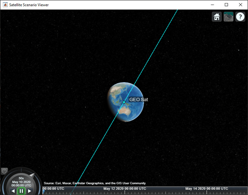
衛星シナリオ ビューアーを使用してシナリオを視覚化します。
v = satelliteScenarioViewer(sc);
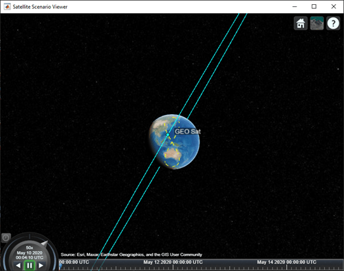
衛星の地上軌跡を視覚化に追加し、地上軌跡の将来と履歴をどの程度表示するかを調整します。
leadTime = 2*24*3600;                                          % seconds
trailTime = leadTime;
gt = groundTrack(sat,"LeadTime",leadTime,"TrailTime",trailTime)
gt =
  GroundTrack with properties:

          LeadTime: 172800
         TrailTime: 172800
         LineWidth: 1
     LeadLineColor: [1 1 0.0670]
    TrailLineColor: [1 1 0.0670]
    VisibilityMode: 'inherit'
衛星の動きと地上での軌跡を視覚化します。衛星は一日のうち半分は日本周辺をカバーし、残りの半分はオーストラリアをカバーします。
play(sc);
バージョン履歴
R2021a で導入
参考
オブジェクト
関数
show|play|groundStation|access|hide|satellite|platform(Satellite Communications Toolbox) |groundTrack