Climate IAM Explorer
| CI Platform | Badges | Results | Coverage |
|---|---|---|---|
| GitHub Actions | TestResults | CodeCoverage |
This repository contains a set of tools to allow users explore integrated assesmemnt models and some examples showcasing how one can use this information in conjuntion to financial applications. The models accessible by the tool include the different datasets hosted by the IIASA Energy program (ENE), but it is extensible to your own custom models. These databases contain a series models that predict the evolution magnitudes including CO2, Energy Prices, and Population among others. Each prediction is based in different climate scenarios established by the model. To understand more about how the different scenarios are built, we recommend visiting the technical documentation for each database. In particular, the links below point the user to the technical documentation for the IAMC1.5 and NGFS datasets.
Huppmann et al., Nature Climate Change (2018)
NGFS Climate Scenarios Database
Please note that this tool is complementary to the more complete (IIASA Scenario Explorer](https://data.ene.iiasa.ac.at/auth/#/) and the main purpose is to allow getting the data directly into MATLAB.
The repository mostly consists of two separate tools. A MATLAB API to the RESTful interface form IIASA below:
https://documenter.getpostman.com/view/1057691/SWE6Zcmd#a361ba3a-9c0b-47f5-be21-58202dd6c804
and a MATLAB App that provides a graphical interface to that same API.
- Using the data explorer App
- Create a Connection
- Exploring the databases
- Working with the IAM Timeseries
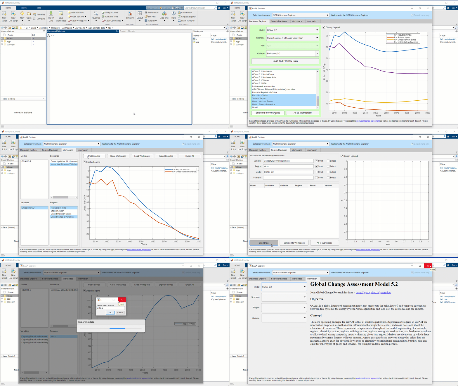
The repository contains a MATLAB app that contains a visual interface to some limited access to the API. For a full "dataset" availability using the programmatic way is probably a better alternative. To Launch the app, you only need to run the command below directly into MATLAB.
IAMDataExplorer
The app will load the NGFS scenario by default, but this can be changed at will.
Programatically, the connection to the IIASA database can be created with a default selected scenario or completely empty. To connect to a specific scenario, please select the product name (e.g. "IXSE_NGFS"), the scheme (e.g. "IXMP Scenario Explorer SPA UI"), the environment (e.g. "ngfs"), or the product name (e.g. "NGFS Scenario Explorer"). For example:
c = iam.data.IIASAConnection('ngfs');
At any point in time, a user can view all the available environments in the database:
c.getEnvironments()
Although the Connection class allows you to perform various REST calls, the best way to explore a database is to use the environment class:
e = iam.IAMEnvironment(c)
This object loads by default all the available Models, Scenarios, Variables, Regions and Runs in the database (not the actual timeseries). For example, you can view all the models by running:
head(e.Variables)
head(e.Models)
The environment also allows you to change the underlying database:
e.changeEnvironment('iamc15');
disp(e)
There are different options to query and select timeseries within the database:
In that case, one can request all the information from the database:
data = e.getTimeSeries('model',"GCAM 5.2",'scenario','Current policies (Hot house world, Rep)')
However, this query can be quite length as there are many different variables and regions that will be requested. Alternatively, the data can be filtered down by "regions" and "variables as:
ts = e.getTimeSeries('model','AIM/CGE 2.0','scenario','ADVANCE_2020_1.5C-2100','regions','World','Variables','Emissions|CO2')
The data returned by the server is always stored in an array of IAM Timeseries objects. Each of these objects will allow you to automatically plot the data by running:
ts.plot('LineWidth');
If neither model or scenario are known, it is also possible to query the data using only the filter values, for example:
e.changeEnvironment('ngfs');

ts = e.getTimeSeries('variables',"Emissions|CO", 'regions', "World");
[ts.Variable]'

ts(1:2).plot();
For simplicity, the legend will only plot those variables that are different in each curve. For example, the previous plot have equal model, scenario, run, and region. So the legend only reports the different variable.
By default, the queries will report any partial match to the dataset you enter. For example, the previous query returned all variables containing Emissions|CO. However, if we wanted a strict match to our inputs we could run:
ts = e.getTimeSeries('variables',"Emissions|CO", 'regions', "World", 'strict',true);
ts(1:2).plot();
The getTimeSeries only accepts a single "strict" command. However, we can still manually filter our results by running:
e.filterVariables('emissions',false)
e.filterVariables('Emissions|CO',true)
This same process can be done with regions
e.filterRegions('japan',false)
e.filterRegions('State of Japan',true)
and with model/scenarios to find out exact runs:
runs = e.filterRuns('model','GCAM','scenario','immediate','strict',false);
e.RunList(ismember(e.RunList.run_id,runs),1:8)
A stack of IAMTimeseries objects can be plot in two main ways: line and bar plots. All plotting functions have two outputs: the array of graphics objects, and the legend.
The data in the object can be plotted as a set of line plots. The plot function accepts the exact same options as the standard plot function in MATLAB. For example:
figure;
ts(1:2).plot('LineWidth',2);
Alternatively, the data in the object can also be plotted as a set of bar plots. The bar funciton accepts the exact same options as the standard bar function in MATLAB.
figure;
[~,l] = ts(1).bar();
l.Location = 'northeast';
One useful utility consists in making a stack plot of several data. For example:
figure;
[h,l] = bar(ts(1:2),'stacked');
l.Location = 'northeast';
引用
Edu Benet Cerda (2024). Climate IAM Explorer (https://github.com/mathworks/Climate-IAM-Explorer/releases/tag/v1.3.4), GitHub. 取得済み .
MATLAB リリースの互換性
プラットフォームの互換性
Windows macOS Linuxタグ
Community Treasure Hunt
Find the treasures in MATLAB Central and discover how the community can help you!
Start Hunting!IAMDataExplorer
IAMDataExplorer/+iam
IAMDataExplorer/+iam/+controls
IAMDataExplorer/+iam/+data
IAMDataExplorer/+iam/+utils
IAMDataExplorer/+iam/+views
IAMDataExplorer/+iam/+views/private
IAMDataExplorer/+iam/@IAMTimeseries
ISMIPExplorer
ISMIPExplorer/+isimip
doc
| バージョン | 公開済み | リリース ノート | |
|---|---|---|---|
| 1.3.4 | See release notes for this release on GitHub: https://github.com/mathworks/Climate-IAM-Explorer/releases/tag/v1.3.4 |
|
|
| 1.3.3.0 | See release notes for this release on GitHub: https://github.com/mathworks/Climate-IAM-Explorer/releases/tag/v1.3.3 |
|
|
| 1.3.2 | See release notes for this release on GitHub: https://github.com/mathworks/Climate-IAM-Explorer/releases/tag/v1.3.2 |
|
|
| 1.3.1 | See release notes for this release on GitHub: https://github.com/mathworks/Climate-IAM-Explorer/releases/tag/v1.3.1 |
|
|
| 1.3.0 | See release notes for this release on GitHub: https://github.com/mathworks/Climate-IAM-Explorer/releases/tag/v1.3.0 |
|
|
| 1.2 | See release notes for this release on GitHub: https://github.com/mathworks/Climate-IAM-Explorer/releases/tag/v1.2 |
|
|
| 1.0.1 | See release notes for this release on GitHub: https://github.com/mathworks/Database-Explorer-for-IIASA/releases/tag/v1.0.1 |
|
|
| 1.0 |
|


