結果:
Our MathWorks Usability Team is working on an accessibility project and they want to interview people who use MATLAB and also have experience with screen readers.
If you fit the criteria and are interested, sign up here https://www.mathworks.com/products/usability.html?tfa_30=A11Y
I wish I knew more about the intended evolution of the capabilities of the function arguments block. I love implementing function syntaxes using this relatively new form, but it doesn't yet handle some function syntax design patterns that I think are valuable and worth keeping.
For example, some functions take an input quantity that can something numeric, or it can be an option string that descriptively names a particular value of that quantity. One example is dateshift(t,"dayofweek",dow), where dow can be an integer from 1 to 7, or it can be one of the option strings "weekday" or "weekend".
Another example is Image Processing Toolbox that take a connectivity specifier as input. The function bwconncomp is one particular case. Connectivity can be specified using certain scalars, certain arrays, or the option string "maximal".
I think this is a worthwhile function design pattern, but I don't think the arguments block validation functionality supports it well (unless you use a lot of extra code that duplicates standard MATLAB behavior, which undermines the value of the arguments block).
MathWorkers - believe me, I know that it is not in your DNA to discuss future features. But would anyone care to offer a hint about directions for the arguments block functionality?

Hi! My name is Mike McLernon, and I’m a product marketing engineer with MathWorks. In my role, I look at the trends ongoing in the wireless industry, across lots of different standards (think 5G, WLAN, SatCom, Bluetooth, etc.), and I seek to shape and guide the software that MathWorks builds to respond to these trends. That’s all about communicating within the Mathworks organization, but every so often it’s worth communicating these trends to our audience in the world at large. Many of the people reading this are engineers (or engineers at heart), and we all want to know what’s happening in the geek world around us. I think that now is one of these times to communicate an important milestone. So, without further ado . . .
Bluetooth 6.0 is here! Announced in September by the Bluetooth Special Interest Group (SIG), it’s making more advances in its quest to create a “world without wires”. A few of the salient features in Bluetooth 6.0 are:
- Channel sounding (for accurate distance measurements)
- Decision-based advertising filtering (for more efficient channel scanning)
- Monitoring advertisers (for improved energy efficiency when devices come into and go out of range)
- Frame space updates (for both higher throughput and better coexistence management)
Bluetooth 6.0 includes other features as well, but the SIG has put special promotional emphasis on channel sounding (CS), which once upon a time was called High Accuracy Distance Measurement (HADM). The SIG has said that CS is a step towards true distance awareness, and 10 cm ranging accuracy. I think their emphasis is in exactly the right place, so let’s learn more about this technology and how it is used.
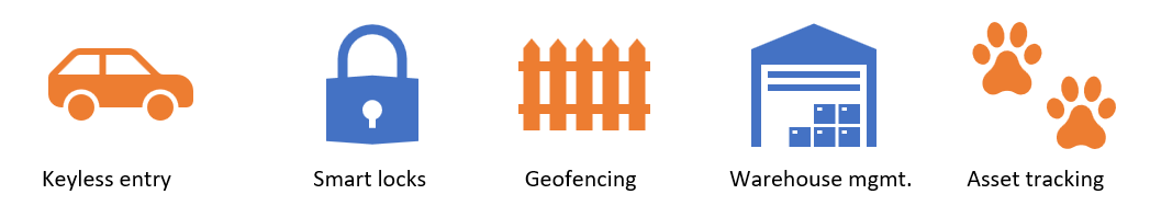
CS can be used for the following use cases:
- Keyless vehicle entry, performed by communication between a key fob or phone and the car’s anchor points
- Smart locks, to permit access only when an authorized device is within a designated proximity to the locks
- Geofencing, to limit access to designated areas
- Warehouse management, to monitor inventory and manage logistics
- Asset tracking for virtually any object of interest
In the past, Bluetooth devices would use a received signal strength indicator (RSSI) measurement to infer the distance between two of them. They would assume a free space path loss on the link, and use a straightforward equation to estimate distance:
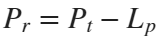
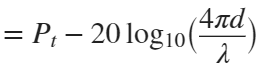
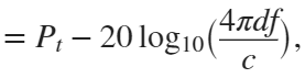 where
whereSo in this method, 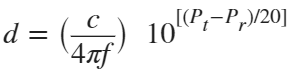 . But if the signal suffers more loss from multipath or shadowing, then the distance would be overestimated. Something better needed to be found.
. But if the signal suffers more loss from multipath or shadowing, then the distance would be overestimated. Something better needed to be found.Bluetooth 6.0 introduces not one, but two ways to accurately measure distance:
- Round-trip time (RTT) measurement
- Phase-based ranging (PBR) measurement
The RTT measurement method uses the fact that the Bluetooth signal time of flight (TOF) between two devices is half the RTT. It can then accurately compute the distance d as
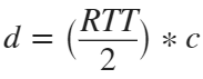 , where c is again the speed of light. This method requires accurate measurements of the time of departure (TOD) of the outbound signal from device 1 (the Initiator), time of arrival (TOA) of the outbound signal to device 2 (the Reflector), TOD of the return signal from device 2, and TOA of the return signal to device 1. The diagram below shows the signal paths and the times.
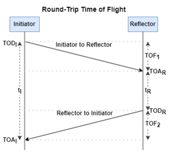
If you want to see how you can use MATLAB to simulate the RTT method, take a look at Estimate Distance Between Bluetooth LE Devices by Using Channel Sounding and Round-Trip Timing.
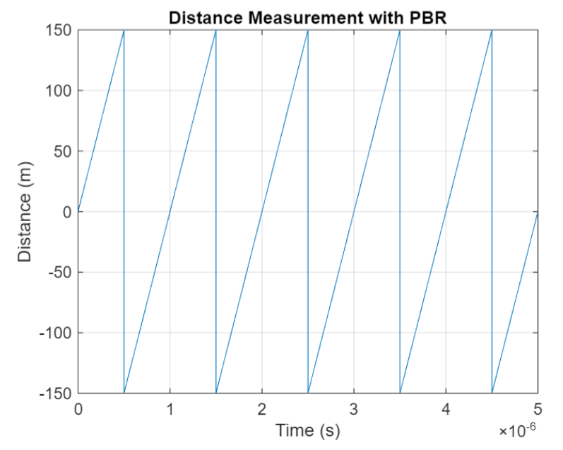
The PBR method uses two Bluetooth signals of different frequencies to measure distance. These signals are simply tones – sine waves. Without going through the derivation, PBR calculates distance d as
The mod() operation is needed to eliminate ambiguities in the distance calculation and the final division by two is to convert a round trip distance to a one-way distance. Because a given phase difference value can hold true for an infinite number of distance values, the mod() operation chooses the smallest distance that satisfies the equation. Also, these tones can be as close as 1 MHz apart. In that case, the maximum resolvable distance measurement is about 150 m. The plot below shows that ambiguity and repetition in distance measurement.
If you want to see how you can use MATLAB to simulate the PBR method, take a look at Estimate Distance Between Bluetooth LE Devices by Using Channel Sounding and Phase-Based Ranging.
Bluetooth 6.0 outlines RTT and PBR distance measurement methods, but CS does not mandate a specific algorithm for calculating distance estimates. This flexibility allows device manufacturers to tailor solutions to various use cases, balancing computational complexity with required accuracy and adapting to different radio environments. Examples include simple phase difference calculations and FFT-based methods.
Although Bluetooth 6.0 is now out, it is far from a finished version. The SIG is actively working through the ratification process for two major extensions:
- High Data Throughput, up to 8 Mbps
- 5 and 6 GHz operation
See the last few minutes of this video from the SIG to learn more about these exciting future developments. And if you want to see more Bluetooth blogs, give a review of this one! Finally, if you have specific Bluetooth questions, give me a shout and let’s start a discussion!
I am very excited to share my new book "Data-driven method for dynamic systems" available through SIAM publishing: https://epubs.siam.org/doi/10.1137/1.9781611978162
This book brings together modern computational tools to provide an accurate understanding of dynamic data. The techniques build on pencil-and-paper mathematical techniques that go back decades and sometimes even centuries. The result is an introduction to state-of-the-art methods that complement, rather than replace, traditional analysis of time-dependent systems. One can find methods in this book that are not found in other books, as well as methods developed exclusively for the book itself. I also provide an example-driven exploration that is (hopefully) appealing to graduate students and researchers who are new to the subject.
Each and every example for the book can be reproduced using the code at this repo: https://github.com/jbramburger/DataDrivenDynSyst
Hope you like it!
Christmas season is underway at my house:

(Sorry - the ornament is not available at the MathWorks Merch Shop -- I made it with a 3-D printer.)
Hi everyone,
I am performing an optimization analysis using MATLAB's Genetic Algorithm (GA) to select design variables, which are then passed to ANSYS to calculate some structural properties. My goal is to find the global optimum, so I have set the population size to 100 × number of variables. While this ensures a broader search space and reduces the risk of getting stuck in local optima, it significantly increases the convergence time because finite element analysis (FEA) needs to be performed for each population member. The current setup takes about a week (or more) to converge, which is not feasible.
To address this, I plan to implement parallel computing for the GA. I need help with the following aspects:
- Parallel Implementation:On my local desktop, I have Number of workers: 6, which means I can evaluate 6 members of the population simultaneously. However, I want to make my code generic so that it automatically adjusts to the number of workers available on any machine. How can I achieve this in MATLAB?
- Improving Convergence Speed:Another approach I’ve come across is using the MigrationInterval and MigrationFractionoptions to divide the population into smaller "islands" that exchange solutions periodically. Would this approach be suitable in my case, and how can I implement it effectively?
- Objective Function Parallelization:Below is the current version of my objective function, which works without parallelization. It writes input variables to an ANSYS .inp file, runs the simulation, and reads results from a text file. How should I modify this function (if needed) to make it compatible with MATLAB’s parallel computing features?
function cost = simple_objective(x, L)
% Write input variables to the file
fid = fopen('Design_Variables.inp', 'w+'); % Ansys APDL reads this
fprintf(fid, 'H_head = %f\n', x(1));
fprintf(fid, 'R_top = %f\n', x(2));
fclose(fid);
% Set ANSYS and Run model
ansys_input = 'ANSYS_APDL.dat';
output_file = 'out_file.txt';
cmd = sprintf('SET KMP_STACKSIZE=15000k & "C:\\Program Files\\ANSYS Inc\\v232\\ansys\\bin\\winx64\\ANSYS232.exe" -b -i %s -o %s', ansys_input, output_file);
system(cmd);
% Remove file lock if it exists
if exist('file.lock', 'file')
delete('file.lock');
end
% Read results
fileID = fopen('PC1.txt', 'r');
load_multip = fscanf(fileID,'%f',[1,inf]);
fclose(fileID);
if load_multip == 0 % nondesignable geometry
cost = 1e9; % penalty
else
cost = -load_multip;
end
end
GA Options:
Here are the GA options I am currently using. Do I need to adjust these for parallelization or migration-based approaches?
“options = optimoptions("ga", ... 'OutputFcn',@SaveOut, ... 'Display', 'iter', ... 'PopulationSize', 200, ... 'Generations', 50, ... 'EliteCount', 2, ... 'CrossoverFraction', 0.98, ... 'TolFun', 1.0e-9, ... 'TolCon', 1.0e-9, ... 'StallTimeLimit', Inf, ... 'FitnessLimit', -Inf, ... 'PlotFcn',{@gaplotbestf,@gaplotstopping});”
I would greatly appreciate it if you could guide me on:
- How to enable and configure parallel computing for GA in MATLAB.
- Any adjustments required in the objective function for parallel execution.
- Whether migration-based GA (using MigrationInterval and MigrationFraction) is a good alternative in my case.
Thank you for your time and help!
So I made this.
clear
close all
clc
% inspired from: https://www.youtube.com/watch?v=3CuUmy7jX6k
%% user parameters
h = 768;
w = 1024;
N_snowflakes = 50;
%% set figure window
figure(NumberTitle="off", ...
name='Mat-snowfalling-lab (right click to stop)', ...
MenuBar="none")
ax = gca;
ax.XAxisLocation = 'origin';
ax.YAxisLocation = 'origin';
axis equal
axis([0, w, 0, h])
ax.Color = 'k';
ax.XAxis.Visible = 'off';
ax.YAxis.Visible = 'off';
ax.Position = [0, 0, 1, 1];
%% first snowflake
ht = gobjects(1, 1);
for i=1:length(ht)
ht(i) = hgtransform();
ht(i).UserData = snowflake_factory(h, w);
ht(i).Matrix(2, 4) = ht(i).UserData.y;
ht(i).Matrix(1, 4) = ht(i).UserData.x;
im = imagesc(ht(i), ht(i).UserData.img);
im.AlphaData = ht(i).UserData.alpha;
colormap gray
end
%% falling snowflake
tic;
while true
% add a snowflake every 0.3 seconds
if toc > 0.3
if length(ht) < N_snowflakes
ht = [ht; hgtransform()];
ht(end).UserData = snowflake_factory(h, w);
ht(end).Matrix(2, 4) = ht(end).UserData.y;
ht(end).Matrix(1, 4) = ht(end).UserData.x;
im = imagesc(ht(end), ht(end).UserData.img);
im.AlphaData = ht(end).UserData.alpha;
colormap gray
end
tic;
end
ax.CLim = [0, 0.0005]; % prevent from auto clim
% move snowflakes
for i = 1:length(ht)
ht(i).Matrix(2, 4) = ht(i).Matrix(2, 4) + ht(i).UserData.velocity;
end
if strcmp(get(gcf, 'SelectionType'), 'alt')
set(gcf, 'SelectionType', 'normal')
break
end
drawnow
% delete the snowflakes outside the window
for i = length(ht):-1:1
if ht(i).Matrix(2, 4) < -length(ht(i).Children.CData)
delete(ht(i))
ht(i) = [];
end
end
end
%% snowflake factory
function snowflake = snowflake_factory(h, w)
radius = round(rand*h/3 + 10);
sigma = radius/6;
snowflake.velocity = -rand*0.5 - 0.1;
snowflake.x = rand*w;
snowflake.y = h - radius/3;
snowflake.img = fspecial('gaussian', [radius, radius], sigma);
snowflake.alpha = snowflake.img/max(max(snowflake.img));
end
Hello,
I have a MATLAB App that has been devolped in the MATLAB App Designer. I have saved all of the apps properties when the user selects the save config menu option and saved it into a .mat file.
Now I want to be able to load this file and update the app to the properties saved in this file. Currently, the program will store the variables in the app structure, but will not update the app's UIFigure. If I save the the UIFigure itself the program will create a new UIFigure and the code in App Designer will no longer work. Hence, why I've added not to save the UIFigure.
if strcmp(propName, 'SuperMarioUIFigure')
continue;
end
Does anyone know how I can get the app structure to update the current UIFigure that App Designer is running?
Here is my current code.
% Menu selected function: SaveConfigMenu
function SaveConfigMenuSelected(app, event)
% Create a structure to hold all the properties of the app
config = struct();
% List all properties of the app
metaProps = properties(app);
% Loop through properties and store their values in structure
for i = 1:length(metaProps)
propName = metaProps{i};
if strcmp(propName, 'SuperMarioUIFigure')
continue;
end
try
config.(propName) = app.(propName);
catch
% Handle any properties that can't be saved
fprintf('Could not save property: %s\n', propName);
end
end
% Prompt user to specify a file to save the configuration
[file, path] = uiputfile('*.mat', 'Save Configuration As');
if isequal(file, 0) || isequal(path, 0)
return; % User cancelled
end
% Save the configuration structure to a file
save(fullfile(path, file), '-struct', 'config');
uialert(app.SuperMarioUIFigure, 'Configuration saved successfully!', 'Save Configuration');
end
% Menu selected function: LoadConfigMenu
function LoadConfigMenuSelected(app, event)
% Prompt user to select a configuration file
[file, path] = uigetfile('*.mat', 'Load Configuration');
if isequal(file, 0) || isequal(path, 0)
return; % User cancelled
end
% Load the configuration structure from the file
config = load(fullfile(path, file));
% List all properties of the app
metaProps = properties(app);
% Update app properties with values from the configuration file
for i = 1:length(metaProps)
propName = metaProps{i};
if isfield(config, propName)
try
app.(propName) = config.(propName);
catch ME
% Handle any properties that can't be updated
fprintf('Could not load property: %s. Error: %s\n', propName, ME.message);
end
end
end
% Display a success message
uialert(app.SuperMarioUIFigure, 'Configuration loaded successfully!', 'Load Configuration');
end
Thanks
Hello, I have a very simple Simulink program to control a servo with my Arduino. The problem is that I'm not getting a full range of the servo. I am using an Adafruit Motor Shield to drive the servo which is a cheap TowerPro. The range I'm getting is 0 to 70. I am using Matlab/Simulink 2019.
Any ideas what could be wrong?
Thank you
The expression for a zero-symmetric polyhedron is known, S={x:[1; 1]<=Ax<=[1; 1]}, where A=[0.5 0; -0.5 0; 0 0.25; 0 -0.25], can you use the polyhedron function to draw an image of the polyhedron, I hope you can write detailed code
Is it possible to differenciate the input, output and in-between wires by colors?
if app.LikeCheckBox.Value==true
app.EditField.Value='you Like our channal'
elseif app.LikeCheckBox.Value==true && app.ShareCheckBox.Value==true
app.EditField.Value='you liked and shared'
elseif app.ShareCheckBox.Value==true
app.EditField.Value='you Share our channal'
elseif app.ShareCheckBox.Value==true && app.SubscribeCheckBox.Value==true
app.EditField.Value='you shared and subscribed'
elseif app.SubscribeCheckBox.Value==true
app.EditField.Value='you Subscribed to our channal'
elseif app.LikeCheckBox.Value==true && app.SubscribeCheckBox.Value==true
app.EditField.Value='good job'
else app.EditField.Value='Choose on item'
app.EditField.HorizontalAlignment='center'
end
At the present time, the following problems are known in MATLAB Answers itself:
- Symbolic output is not displaying. The work-around is to disp(char(EXPRESSION)) or pretty(EXPRESSION)
- Symbolic preferences are sometimes set to non-defaults
Hello, MATLAB fans!
For years, many of you have expressed interest in getting your hands on some cool MathWorks merchandise. I'm thrilled to announce that the wait is over—the MathWorks Merch Shop is officially open!

In our shop, you'll find a variety of exciting items, including baseball caps, mugs, T-shirts, and YETI bottles.
Visit the shop today and explore all the fantastic merchandise we have to offer. Happy shopping!
I was curious to startup your new AI Chat playground.
The first screen that popped up made the statement:
"Please keep in mind that AI sometimes writes code and text that seems accurate, but isnt"
Can someone elaborate on what exactly this means with respect to your AI Chat playground integration with the Matlab tools?
Are there any accuracy metrics for this integration?
Just shared an amazing YouTube video that demonstrates a real-time PID position control system using MATLAB and Arduino.
When I am inputting data, I am trying to input an equation that I should result in multiple answers. The equation I am trying to do is an output in Kw, divided by a conversion percentage. That percentage ranges from 5-15. No matter what way I put this data in to the system, it kicks out a bunch of 0's and then one column of real numners. The data chart should be 5 columns wide and 11 rows down, but for some reason it is giving me excess columns. 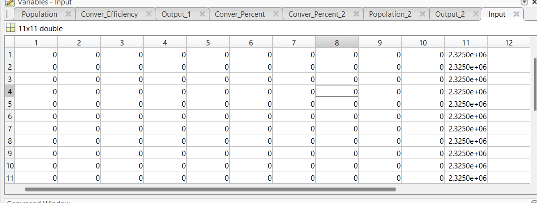
I don't like the change
16%
I really don't like the change
29%
I'm okay with the change
24%
I love the change
11%
I'm indifferent
11%
I want both the web & help browser
11%
38 票
We are thrilled to announce the grand prize winners of our MATLAB Shorts Mini Hack contest! This year, we invited the MATLAB Graphics and Charting team, the authors of the MATLAB functions used in every entry, to be our judges. After careful consideration, they have selected the top three winners:
Judge comments: Realism & detailed comments; wowed us with Manta Ray
2nd place – Jenny Bosten
Judge comments: Topical hacks : Auroras & Wind turbine; beautiful landscapes & nightscapes
3rd place - Vasilis Bellos
Judge comments: Nice algorithms & extra comments; can’t go wrong with Pumpkins
Judge comments: Impressive spring & cubes!
In addition, after validating the votes, we are pleased to announce the top 10 participants on the leaderboard:
Congratulations to all! Your creativity and skills have inspired many of us to explore and learn new skills, and make this contest a big success!