メインコンテンツ
結果:
The study of nonlinear dynamical systems in lattices is an area of research with continuously growing interest.The first systematic studies of these systems emerged in the late 1930 s,thanks to the work of Frenkel and Kontorova on crystal dislocations.These studies led to the formulation of the discrete Klein-Gordon equation (DKG).Specifically,in 1939,Frenkel and Kontorova proposed a model that describes the structure and dynamics of a crystal lattice in a dislocation core.The FK model has become one of the fundamental models in physics,as it has been proven to reliably describe significant phenomena observed in discrete media.The equation we will examine is a variation of the following form:
The process described involves approximating a nonlinear differential equation through the Taylor method and simplifying it into a linear model.Let's analyze step by step the process from the initial equation to its final form.For small angles, can be approximated through the Taylor series as:
We substitute  in the original equation with the Taylor approximation:
To map this equation to a linear model,we consider the angles  to correspond to displacements
  in a mass-spring system.Thus,the equation transforms into:
 to correspond to displacements
 We recognize that the term  expresses the nonlinearity of the system,while β is a coefficient corresponding to this nonlinearity,simplifying the expression.The final form of the equation is:
The exact value of β depends on the mapping of coefficients in the Taylor approximation and its application to the specific physical problem.Our main goal is to derive results regarding stability and convergence in nonlinear lattices under nonlinear conditions.We will examine the basic characteristics of the discrete Klein-Gordon equation:
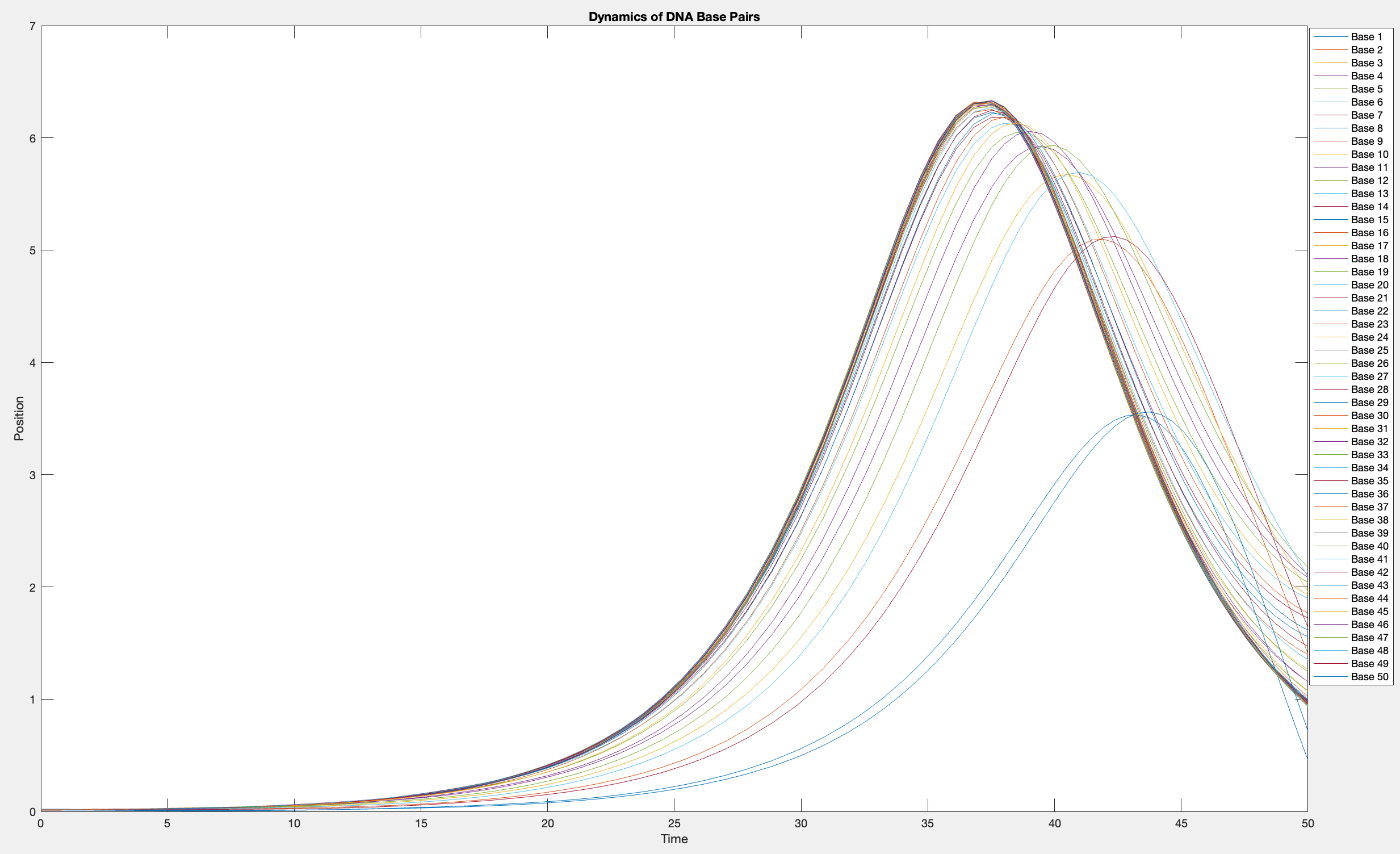
This model is often used to describe the opening of the DNA double helix during processes such as transcription.The model focuses on the transverse motion of the base pairs,which can be represented by a set of coupled nonlinear differential equations.
% Parameters
numBases = 50; % Number of base pairs
kappa = 0.1; % Elasticity constant
omegaD = 0.2; % Frequency term
beta = 0.05; % Nonlinearity coefficient
% Initial conditions
initialPositions = 0.01 + (0.02 - 0.01) * rand(numBases, 1);
initialVelocities = zeros(numBases, 1);
Time span
tSpan = [0 50];
>> % Differential equations
odeFunc = @(t, y) [y(numBases+1:end); ... % velocities
kappa * ([y(2); y(3:numBases); 0] - 2 * y(1:numBases) + [0; y(1:numBases-1)]) + ...
omegaD^2 * (y(1:numBases) - beta * y(1:numBases).^3)]; % accelerations
% Solve the system
[T, Y] = ode45(odeFunc, tSpan, [initialPositions; initialVelocities]);
% Visualization
plot(T, Y(:, 1:numBases))
legend(arrayfun(@(n) sprintf('Base %d', n), 1:numBases, 'UniformOutput', false))
xlabel('Time')
ylabel('Position')
title('Dynamics of DNA Base Pairs')
% Choose a specific time for the snapshot
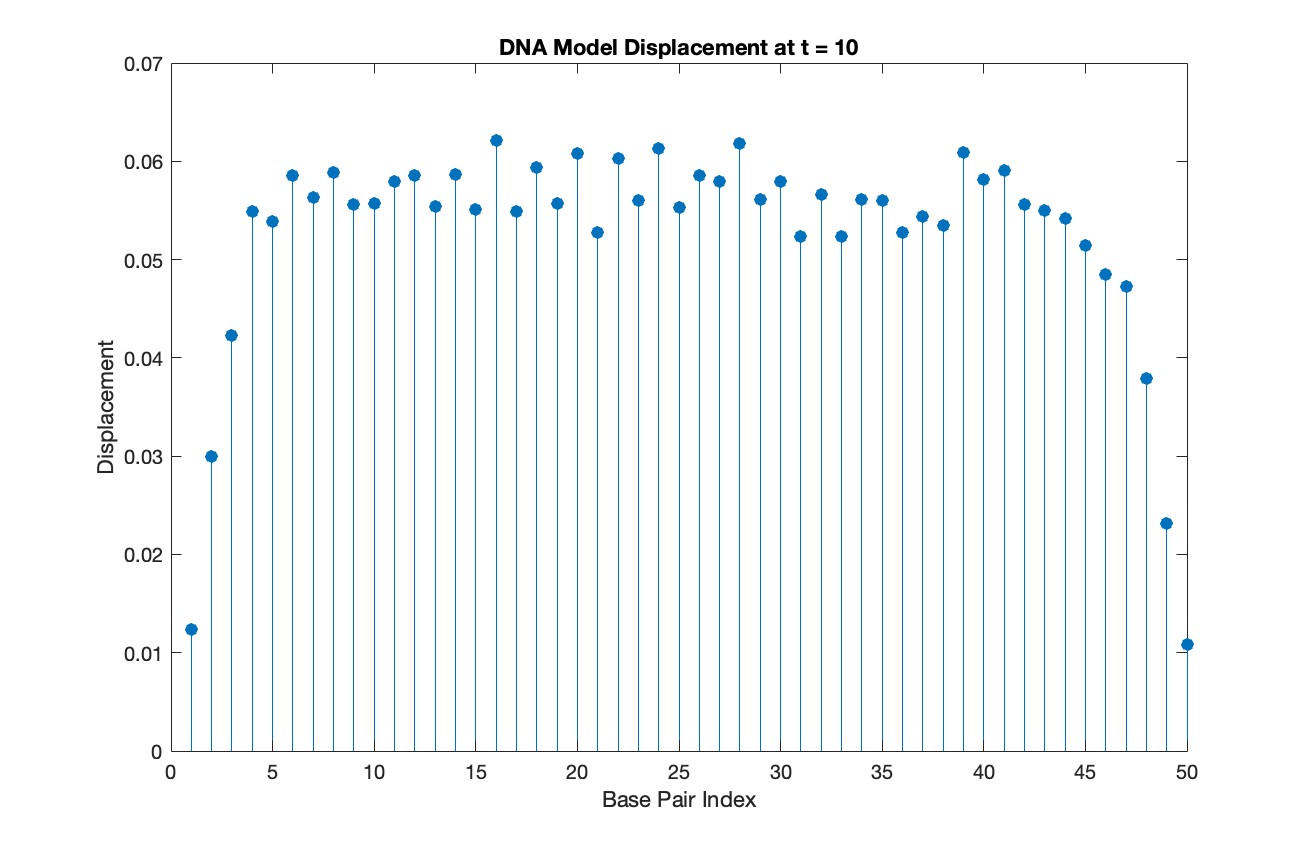
snapshotTime = 10;
% Find the index in T that is closest to the snapshot time
[~, snapshotIndex] = min(abs(T - snapshotTime));
% Extract the solution at the snapshot time
snapshotSolution = Y(snapshotIndex, 1:numBases);
% Generate discrete plot for the DNA model at the snapshot time
figure;
stem(1:numBases, snapshotSolution, 'filled')
title(sprintf('DNA Model Displacement at t = %d', snapshotTime))
xlabel('Base Pair Index')
ylabel('Displacement')
% Time vector for detailed sampling
tDetailed = 0:0.5:50;
% Initialize an empty array to hold the data
data = [];
% Generate the data for 3D plotting
for i = 1:numBases
% Interpolate to get detailed solution data for each base pair
detailedSolution = interp1(T, Y(:, i), tDetailed);
% Concatenate the current base pair's data to the main data array
data = [data; repmat(i, length(tDetailed), 1), tDetailed', detailedSolution'];
end
% 3D Plot
figure;
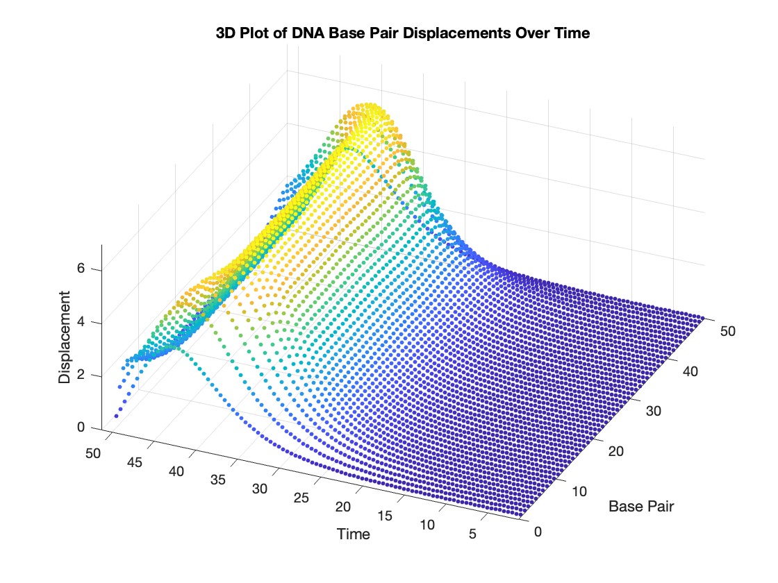
scatter3(data(:,1), data(:,2), data(:,3), 10, data(:,3), 'filled')
xlabel('Base Pair')
ylabel('Time')
zlabel('Displacement')
title('3D Plot of DNA Base Pair Displacements Over Time')
colormap('rainbow')
colorbar
Lots of students like me have a break from school this week or next! If y'all are looking for something interesting to do learn a bit about using hgtransform by making the transforming snake animation in MATLAB!
Code below!
⬇️⬇️⬇️
numblock=24;
v = [ -1 -1 -1 ; 1 -1 -1 ; -1 1 -1 ; -1 1 1 ; -1 -1 1 ; 1 -1 1 ];
f = [ 1 2 3 nan; 5 6 4 nan; 1 2 6 5; 1 5 4 3; 3 4 6 2 ];
clr = hsv(numblock);
shapes = [ 1 0 0 0 0 0 1 0 0 0 0 1 0 0 0 0 0 0 1 0 0 0 0 1 % box
0 0 .5 -.5 .5 0 1 0 -.5 .5 -.5 0 1 0 .5 -.5 .5 0 1 0 -.5 .5 -.5 0 % fluer
0 0 1 1 0 .5 -.5 1 .5 .5 -.5 -.5 1 .5 .5 -.5 -.5 1 .5 .5 -.5 -.5 1 .5 % bowl
0 .5 -.5 -.5 .5 -.5 .5 .5 -.5 .5 -.5 -.5 .5 -.5 .5 .5 -.5 .5 -.5 -.5 .5 -.5 .5 .5]; % ball
% Build the assembly
set(gcf,'color','black');
daspect(newplot,[1 1 1]);
xform=@(R)makehgtform('axisrotate',[0 1 0],R,'zrotate',pi/2,'yrotate',pi,'translate',[2 0 0]);
P=hgtransform('Parent',gca,'Matrix',makehgtform('xrotate',pi*.5,'zrotate',pi*-.8));
for i = 1:numblock
P = hgtransform('Parent',P,'Matrix',xform(shapes(end,i)*pi));
patch('Parent',P, 'Vertices', v, 'Faces', f, 'FaceColor',clr(i,:),'EdgeColor','none');
patch('Parent',P, 'Vertices', v*.75, 'Faces', f(end,:), 'FaceColor','none',...
'EdgeColor','w','LineWidth',2);
end
view([10 60]);
axis tight vis3d off
camlight
% Setup vectors for animation
h=findobj(gca,'type','hgtransform')'; h=h(2:end);
r=shapes(end,:)*pi;
steps=100;
% Animate between different shapes
for si = 1:size(shapes,1)
sh = shapes(si,:)*pi;
diff = (sh-r)/steps;
% Animate to a new shape
for s=1:steps
arrayfun(@(tx)set(h(tx),'Matrix',xform(r(tx)+diff(tx)*s)),1:numblock);
view([s*360/steps 20]); drawnow();
end
r=sh;
for s=1:steps; view([s*360/steps 20]); drawnow(); end % finish rotate
end
I asked my question in the general forum and a few minutes later it was deleted. Perhaps this is a better place?
Rather than using my German regional forum (as I do not speak German), I want to ask questions in an international English-speaking forum. Presumably there should be an international English forum for everyone around the world, as English is the first or second language of everyone who has gone to school. Where is it?
I was looking into the possibility of making a spin-to-win prize wheel in MATLAB. I was looking around, and if someone has made one before they haven't shared. A labeled colored spinning wheel, that would slow down and stop (or I would take just stopping) at a random spot each time. I would love any tips or links to helpful resources!
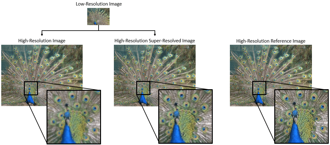
Many of the examples in the MATLAB documentation are extremely high quality articles, often worthy of attention in their own right. Time to start celebrating them! Today's is how to increase Image Resolution using deep learning
https://uk.mathworks.com/help/deeplearning/ug/single-image-super-resolution-using-deep-learning.html
Struct is an easy way to combine different types of variants. But now MATLAB supports classes well, and I think class is always a better alternative than struct. I can't find a single scenario that struct is necessary. There are many shortcomings using structs in a project, e.g. uncontrollable field names, unexamined values, etc. What's your opinion?
I am confused, is the matlab answer better or Julia’s?
Hello and a warm welcome to all! We're thrilled to have you visit our community. MATLAB Central is a place for learning, sharing, and connecting with others who share your passion for MATLAB and Simulink. To ensure you have the best experience, here are some tips to get you started:
- Read the Community Guidelines: Understanding our community standards is crucial. Please take a moment to familiarize yourself with them. Keep in mind that posts not adhering to these guidelines may be flagged by moderators or other community members.
- Ask Technical Questions at MATLAB Answers: If you have questions related to MathWorks products, head over to MATLAB Answers (new question form - Ask the community). It's the go-to spot for technical inquiries, with responses often provided within an hour, depending on the complexity of the question and volunteer availability. To increase your chances of a speedy reply, check out our tips on how to craft a good question (link to post on asking good questions).
- Choosing the Right Channel: We offer a variety of discussion channels tailored to different contexts. Select the one that best fits your post. If you're unsure, the General channel is always a safe bet. If you feel there's a need for a new channel, we encourage you to suggest it in the Ideas channel.
- Reporting Issues: If you encounter posts that violate our guidelines, please use the 🚩Flag/Report feature (found in the 3-dot menu) to bring them to our attention.
- Quality Control: We strive to maintain a high standard of discussion. Accounts that post spam or too much nonsense may be subject to moderation, which can include temporary suspensions or permanent bans.
- Share Your Ideas: Your feedback is invaluable. If you have suggestions on how we can improve the community or MathWorks products, the Ideas channel is the perfect place to voice your thoughts.
Enjoy yourself and have fun! We're committed to fostering a supportive and educational environment. Dive into discussions, share your expertise, and grow your knowledge. We're excited to see what you'll contribute to the community!
Have you ever used Live Tasks in MATLAB? MathWorks development team would like to get some feedback on your experience – what did you like and not like. Especially, if you know about it but don’t use it frequently, we would like to understand why?
Please tell us what you think by submitting your response to this form https://forms.office.com/r/ui1EGqAFDx
MathWorks just released three new courses on Coursera liseted below. If you work with image or video data and are wanting to incorporate deep learning techniques into your workflow, this is a great opporutnity. The course creators monitor the discussion forums, so you can ask questions and get feedback on your work. Below are links to the three courses and a quick description of a project you'll complete in each.
- Introduction to Computer Vision for Deep Learning. You'll train a classifier to classify images of people signing the American Sign Language alphabet.
- Deep Learning for Object Detection. Move from just classification to finding object locations. You'll train a model to find different types of parking available on the MathWorks campus.
- Advanced Deep Learning Techniques for Computer Vision. You'll train anomaly detection models for medical images and use AI-assisted labeling auto label images.
Can anyone provide insight into the intended difference between Discussions and Answers and what should be posted where?
Just scrolling through Discussions, I saw postst that seem more suitable Answers?
What exactly does Discussions bring to the table that wasn't already brought by Answers?
Maybe this question is more suitable for a Discussion ....
Hello Community!
We are working on a new translation experience for the MathWorks website and products. The goal is to make it easy for people to see content in the best language for them.
Step 1 is learning from those of you who use another language instead of, or in addition to English. If this sounds like you, we'd love your response to a brief survey.
Feel free to comment here as well. Thanks in advance!
We've released an open-source implementation of STIPA (Speech Transmission Index for Public Address) on GitHub!
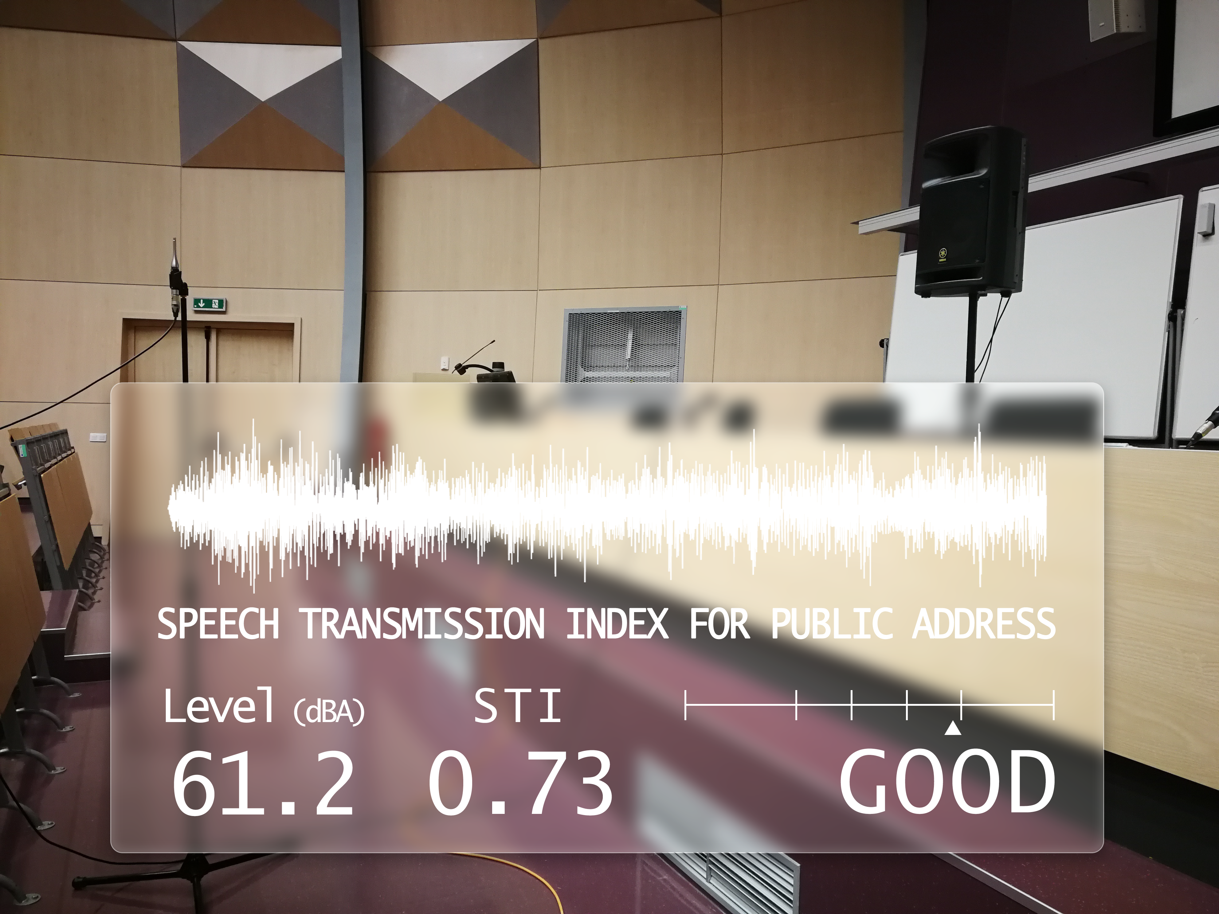
What is STIPA?
Speech Transmission Index is a metric designed to assess the quality of speech transmission through a communication channel. It quantifies the intelligibility of speech signals based on amplitude modulations, providing a standardized measure crucial for evaluating public address systems and communication equipment. STIPA is a version of STI using a simplified measurement method and only one test signal.
Quality Representation:
STI values range from 0 to 1, categorizing speech transmission quality from bad to excellent. The raw STI score can be transformed into the likelihood of intelligibility of syllables, words, and sentences being comprehended.
Verification Tests:
To ensure reliability, we've conducted verification tests according to the IEC 60286-16 standard. Download the test signals and run the stipaVerificationTests.m script from our GitHub repository.
Control Measurements:
We've performed comparative measurements in a university auditorium, showcasing the validity of our implementation.
License:
Our STIPA implementation is distributed under the GNU General Public License 3, reflecting our commitment to open-source collaboration.
i am just thinking to make a project on software defined ratio SDR using matlab and its toolboxes but I am UG student in ECE don't know how to start can we have discussion here and want the guidance from the best or good persons in the field of wireless communication
I noticed a couple new replies show up on the recent poll a day or so ago, but since then, the page can't be loaded anymore in any browser I've tried.

Is MathWorks going to spend 5 years starting in 2024 making Python the #1 supported language?
I'm not sure it's authentic information, and am looking forward to a high level of integration with python.
Reference:
Hello, I am a student and I am working on a neural network for a line follower car and I would like you to recommend a tutorial to implement it in simulink.
good afternoon everyone my name is Dundu lawan haruna ,i'm a final year student at the department of computer engineering ABU Zaria, Nigerian , and i wanted to do my final year project based on computer vision : project topic , designing an eye glasses to help those people with visual imparement to be able to navigate enviroment efficiently , that's why i need a support from you guys ,all advised are highly well come , thank you for your support.
Recently, I came across a post about the JIT compiler on this Korean blog. In the post. The writer discussed the concept of the "Compile Threshold" and how it is calculated.
"The JVM accumulates the number of calls for each method called and compiles when the number exceeds a certain number. In other words, there is a standard for checking how often it is called and then deciding, 'It is time to compile.' This standard is called the compilation threshold. But what is this and why should it be used as a standard?"
The concept of the "Compile Threshold," as used above, seems to be more commonly associated with Tracing just-in-time compilation.
The writer used the simple Java code below to calculate the threshold.
for (int i = 0; i < 500; ++i) {
long startTime = System.nanoTime();
for (int j = 0; j < 1000; ++j) {
new Object();
}
long endTime = System.nanoTime();
System.out.printf("%d\t%d\n", i, endTime - startTime);
}
Since the MATLAB execution engine uses JIT compilation, I just wanted to perform the same experiment that the writer did.
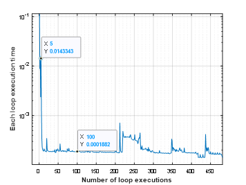
I experimented using simple codes based on the code in the blog. I iterated a function 500 time using for-loop and calculated the execution time for each iteration using tic and toc. Then I plotted the execution time for each loop as blow. First five execution times are much higher than followings (10 times!) The test is very rough so I am not sure that I can conclude "MATLAB has Compile Threshold and it is 5!" but this value is actually correct ;-)
t0 = 0;
tfinal = 10;
y0 = [20;20];
timeToRun = zeros(500,1);
for i = 1:500
tStart = tic;
[preypeaks,predatorpeaks] = solvelotka(t0, tfinal, y0);
tEnd = toc(tStart);
timeToRun(i) = tEnd;
end
VS Code Extension for MATLAB was introduced back in April and has been downloaded 75K times since. Do people here use VS Code for writing MATLAB code?


