結果:
Check out the LLMs with MATLAB project on File Exchange to access Large Language Models from MATLAB.
Along with the latest support for GPT-4o mini, you can use LLMs with MATLAB to generate images, categorize data, and provide semantic analyis.
function ans = your_fcn_name(n)
n;
j=sum(1:n);
a=zeros(1,j);
for i=1:n
a(1,((sum(1:(i-1))+1)):(sum(1:(i-1))+i))=i.*ones(1,i);
end
disp
I am trying to earn my Intro to MATLAB badge in Cody, but I cannot click the Roll the Dice! problem. It simply is not letting me click it, therefore I cannot earn my badge. Does anyone know who I should contact or what to do?
I define the class in matlab as:
classdef Myclass
properties
Content
end
methods
function obj = Myclass(content)
obj.Content = content;
end
function disp(obj)
A = symmatrix('A(1/3,[0,0,1])');
disp(A);
end
end
end
When we run this class in live editor return 'A(1/3,[0,0,1])' rather than latex form.
Myclass(1)
% return 'A(1/3,[0,0,1])'
A = symmatrix('A(1/3,[0,0,1])');
% return latrx form A(1/3,[0,0,1])
Something that had bothered me ever since I became an FEA analyst (2012) was the apparent inability of the "camera" in Matlab's 3D plot to function like the "cameras" in CAD/CAE packages.
For instance, load the ForearmLink.stl model that ships with the PDE Toolbox in Matlab and ParaView and try rotating the model.
clear
close all
gm = importGeometry( "ForearmLink.stl" );
pdegplot(gm)
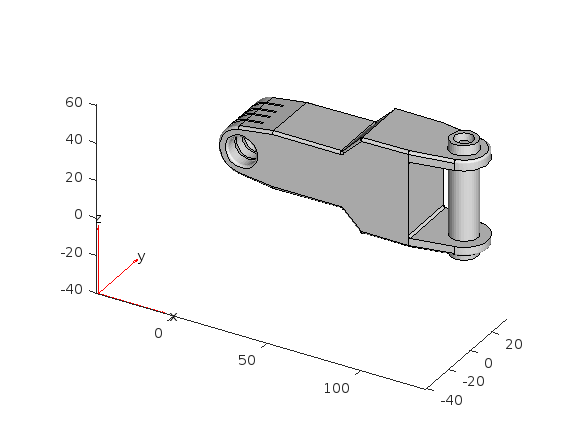
Things to observe:
- Note that I cant seem to rotate continuously around the x-axis. It appears to only support rotations from [0, 360] as opposed to [-inf, inf]. So, for example, if I'm looking in the Y+ direction and rotate around X so that I'm looking at the Z- direction, and then want to look in the Y- direction, I can't simply keep rotating around the X axis... instead have to rotate 180 degrees around the Z axis and then around the X axis. I'm not aware of any data visualization applications (e.g., ParaView, VisIt, EnSight) or CAD/CAE tools with such an interaction.
- Note that at the 50 second mark, I set a view in ParaView: looking in the [X-, Y-, Z-] direction with Y+ up. Try as I might in Matlab, I'm unable to achieve that same view perspective.
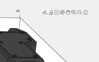
Today I discovered that if one turns on the Camera Toolbar from the View menubar, then clicks the Orbit Camera icon, then the No Principal Axis icon:
That then it acts in the manner I've long desired. Oh, and also, for the interested, it is programmatically available: https://www.mathworks.com/help/matlab/ref/cameratoolbar.html
I might humbly propose this mode either be made more discoverable, similar to the little interaction widgets that pop up in figures:
Or maybe use the middle-mouse button to temporarily use this mode (a mouse setting in, e.g., Abaqus/CAE).
I've noticed is that the highly rated fonts for coding (e.g. Fira Code, Inconsolata, etc.) seem to overlook one issue that is key for coding in Matlab. While these fonts make 0 and O, as well as the 1 and l easily distinguishable, the brackets are not. Quite often the curly bracket looks similar to the curved bracket, which can lead to mistakes when coding or reviewing code.
So I was thinking: Could Mathworks put together a team to review good programming fonts, and come up with their own custom font designed specifically and optimized for Matlab syntax?
could you explain me how to calculate the gain values for different types of controllers (Conventional Sliding Mode Control, Third Order Sliding Mode Control, Variable Gain Super Twisting Algorithm.
Could you, assist me in providing a mathematical method, for example, to calculate the gains of the above-mentioned controllers?
Thank you
M. Itouchene
Hi,
I'm trying to write a code which can determine the gradient change in a given profile. However the code is unable to determine the same correctly and giving incorrect results. For the pic1 below it should give me the width of the region where it is a steep gradient determined.
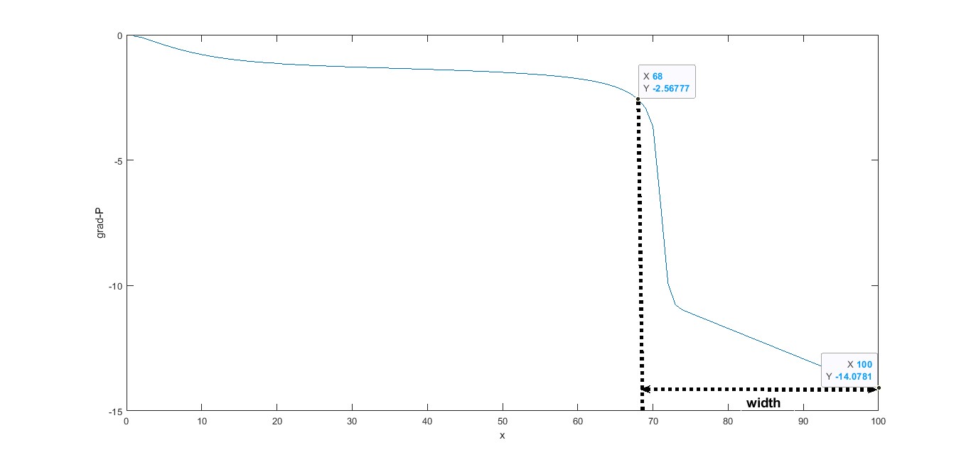
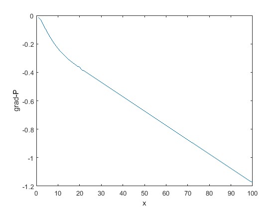
However for pic2 below it shouldn't as there is no steep gradient compared to pic1
The code is as below:
clear width;
global width;
global data;
for i=1:max(length(data.variable.t))
for j=1:max(length(data.variable.x))-1
change_p = (abs(data.variable.gradpressure(i,j+1))-abs(data.variable.gradpressure(i,j)))/abs(data.variable.gradpressure(i,j));
%disp(change_p)
if change_p > 0.1
disp("steep gradient found")
width(j)=1-data.variable.x(j);
disp(width)
else
disp("no steep gradient found")
end
end
end
the data.variable.gradpressure is a 1000x100 matrix with t along the vertical and x along the horizontal.
with regards,
rc
Sub aspenaAdorption()
' Declare variables for the ACM application, document, and simulation
Dim ACMApp As Object
Dim ACMDocument As Object
Dim ACMSimulation As Object
' Create an instance of the ACM application
Set ACMApp = CreateObject("ACM Application")
' Use "ACM Application" for Aspen Custom Modeler
' Use "ADS Application" for Aspen Adsorption
' Make the ACM application visible
ACMApp.Visible = True
' Open the specified simulation document
Set ACMDocument = ACMApp.OpenDocument("C:\Users\user\Desktop\H2_Purification.acmf")
' Set the simulation object to the current simulation in the application
Set ACMSimulation = ACMApp.Simulation
' Set the simulation to run in dynamic mode
ACMSimulation.RunMode = "Dynamic"
' Run the simulation
ACMSimulation.Run (True)
' Check if the simulation was successful and display a message box
If ACMSimulation.Successful Then
MsgBox "Simulation Complete"
Else
MsgBox "Simulation Failed"
End If
' Quit the ACM application
ACMApp.Quit
End Sub
I have an old application that gives me an error when I run it. The error message states: "Could not find version 7.13 of the MCR. Attempting to load mclmcrrt713.dll. Please install the correct version of the MCR." I tried to install this version, but it is no longer available. Any help would be highly appreciated. Thanks!
In the program given below I fail to obtaine real pole as title in intger format if anyone know please guide me
num1=[1 -1];
den1=conv([1 1],conv([1 2+2j],[1 2-2j]));
G=tf(num1,den1);
P=pole(G);
Z = zero(G);
formatSpec='%s,%i,%f+%fi,%i';
a="Root Locus of ";
b='step response of';
figure(17)
rlocus(G)
p=sprintf(formatSpec,a,Z,P/1i,P(3,1));
title(p);
Hi,
I have a condition where at the left boundary and the right boundary I need the flux to be non-zero.
Thus, the equations
pL + qL*fL = 0 and pr + qr*fr = 0 are such that fL and fr being non zero is making my equation hard to determine the values for pl, ql as well as pr, qr.
Plz tell me how should I approach for the same.
with regards,
rc
An option for 10th degree polynomials but no weighted linear least squares. Seriously? Jesse
What do you think about the NVIDIA's achivement of becoming the top giant of manufacturing chips, especially for AI world?

Hello, everyone! I’m Mark Hayworth, but you might know me better in the community as Image Analyst. I've been using MATLAB since 2006 (18 years). My background spans a rich career as a former senior scientist and inventor at The Procter & Gamble Company (HQ in Cincinnati). I hold both master’s & Ph.D. degrees in optical sciences from the College of Optical Sciences at the University of Arizona, specializing in imaging, image processing, and image analysis. I have 40+ years of military, academic, and industrial experience with image analysis programming and algorithm development. I have experience designing custom light booths and other imaging systems. I also work with color and monochrome imaging, video analysis, thermal, ultraviolet, hyperspectral, CT, MRI, radiography, profilometry, microscopy, NIR, and Raman spectroscopy, etc. on a huge variety of subjects.
I'm thrilled to participate in MATLAB Central's Ask Me Anything (AMA) session, a fantastic platform for knowledge sharing and community engagement. Following Adam Danz’s insightful AMA on staff contributors in the Answers forum, I’d like to discuss topics in the area of image analysis and processing. I invite you to ask me anything related to this field, whether you're seeking recommendations on tools, looking for tips and tricks, my background, or career development advice. Additionally, I'm more than willing to share insights from my experiences in the MATLAB Answers community, File Exchange, and my role as a member of the Community Advisory Board. If you have questions related to your specific images or your custom MATLAB code though, I'll invite you to ask those in the Answers forum. It's a more appropriate forum for those kinds of questions, plus you can get the benefit of other experts offering their solutions in addition to me.
For the coming weeks, I'll be here to engage with your questions and help shed light on any topics you're curious about.
Hello, everyone!
Over the past few weeks, our community has been buzzing with activity, showcasing the incredible depth of knowledge, creativity, and innovation that makes this forum such a vibrant place. Today, we're excited to highlight some of the noteworthy contributions that have sparked discussions, offered insights, and shared knowledge across various topics. Let's dive in!
Interesting Questions
Fatima Majeed brings us a thought-provoking mathematical challenge, delving into inequalities and the realms beyond (e^e). If you're up for a mathematical journey, this question is a must-see!
lil brain tackles a practical problem many of us have faced: efficiently segmenting a CSV file based on specific criteria. This post is not only a query but a learning opportunity for anyone dealing with similar data manipulation challenges.
Popular Discussions
Discover a simple yet effective trick for digit manipulation from goc3. This tip is especially handy for those frequenting Cody challenges or anyone interested in enhancing their number handling skills in MATLAB.
Chen Lin shares an exciting update about the 'Run Code' feature in the Discussions area, highlighting how our community can now directly execute and share code snippets within discussions. This feature marks a significant enhancement in how we interact and solve problems together.
From the Blogs
A Deep Dive into EEG Analysis for Predicting Neurological Outcomes By Tanya Kuruvilla
Connell D`Souza, alongside Team Swarthbeat, explores the cutting-edge application of EEG analysis in predicting neurological outcomes post-cardiac arrest. This blog post offers an in-depth look into the challenges and methodologies of modern medical data analysis.
Mihir Acharya discusses the pivotal role of MATLAB and Simulink in the future of robotics simulation. Through an engaging conversation with industry analyst George Chowdhury, this post sheds light on overcoming simulation challenges and the exciting possibilities that lie ahead.
We encourage everyone to explore these contributions further and engage with the authors and the community. Your participation is what fuels this community's continual growth and innovation.
Here's to many more discussions, discoveries, and breakthroughs together!
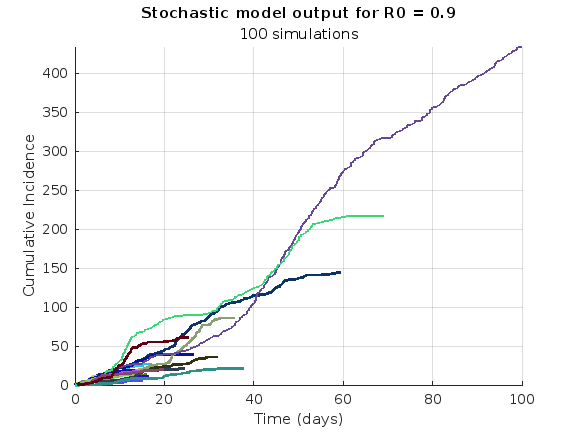
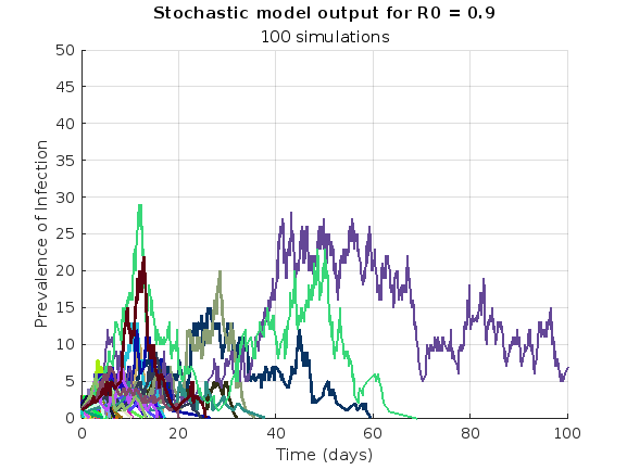
We are modeling the introduction of a novel pathogen into a completely susceptible population. In the cells below, I have provided you with the Matlab code for a simple stochastic SIR model, implemented using the "GillespieSSA" function
Simulating the stochastic model 100 times for 
Since γ is 0.4 per day,  per day
% Define the parameters
beta = 0.36;
gamma = 0.4;
n_sims = 100;
tf = 100; % Time frame changed to 100
% Calculate R0
R0 = beta / gamma
% Initial state values
initial_state_values = [1000000; 1; 0; 0]; % S, I, R, cum_inc
% Define the propensities and state change matrix
a = @(state) [beta * state(1) * state(2) / 1000000, gamma * state(2)];
nu = [-1, 0; 1, -1; 0, 1; 0, 0];
% Define the Gillespie algorithm function
function [t_values, state_values] = gillespie_ssa(initial_state, a, nu, tf)
t = 0;
state = initial_state(:); % Ensure state is a column vector
t_values = t;
state_values = state';
while t < tf
rates = a(state);
rate_sum = sum(rates);
if rate_sum == 0
break;
end
tau = -log(rand) / rate_sum;
t = t + tau;
r = rand * rate_sum;
cum_sum_rates = cumsum(rates);
reaction_index = find(cum_sum_rates >= r, 1);
state = state + nu(:, reaction_index);
% Update cumulative incidence if infection occurred
if reaction_index == 1
state(4) = state(4) + 1; % Increment cumulative incidence
end
t_values = [t_values; t];
state_values = [state_values; state'];
end
end
% Function to simulate the stochastic model multiple times and plot results
function simulate_stoch_model(beta, gamma, n_sims, tf, initial_state_values, R0, plot_type)
% Define the propensities and state change matrix
a = @(state) [beta * state(1) * state(2) / 1000000, gamma * state(2)];
nu = [-1, 0; 1, -1; 0, 1; 0, 0];
% Set random seed for reproducibility
rng(11);
% Initialize plot
figure;
hold on;
for i = 1:n_sims
[t, output] = gillespie_ssa(initial_state_values, a, nu, tf);
% Check if the simulation had only one step and re-run if necessary
while length(t) == 1
[t, output] = gillespie_ssa(initial_state_values, a, nu, tf);
end
if strcmp(plot_type, 'cumulative_incidence')
plot(t, output(:, 4), 'LineWidth', 2, 'Color', rand(1, 3));
elseif strcmp(plot_type, 'prevalence')
plot(t, output(:, 2), 'LineWidth', 2, 'Color', rand(1, 3));
end
end
xlabel('Time (days)');
if strcmp(plot_type, 'cumulative_incidence')
ylabel('Cumulative Incidence');
ylim([0 inf]);
elseif strcmp(plot_type, 'prevalence')
ylabel('Prevalence of Infection');
ylim([0 50]);
end
title(['Stochastic model output for R0 = ', num2str(R0)]);
subtitle([num2str(n_sims), ' simulations']);
xlim([0 tf]);
grid on;
hold off;
end
% Simulate the model 100 times and plot cumulative incidence
simulate_stoch_model(beta, gamma, n_sims, tf, initial_state_values, R0, 'cumulative_incidence');
% Simulate the model 100 times and plot prevalence
simulate_stoch_model(beta, gamma, n_sims, tf, initial_state_values, R0, 'prevalence');
Twitch built an entire business around letting you watch over someone's shoulder while they play video games. I feel like we should be able to make at least a few videos where we get to watch over someone's shoulder while they solve Cody problems. I would pay good money for a front-row seat to watch some of my favorite solvers at work. Like, I want to know, did Alfonso Nieto-Castonon just sit down and bang out some of those answers, or did he have to think about it for a while? What was he thinking about while he solved it? What resources was he drawing on? There's nothing like watching a master craftsman at work.
I can imagine a whole category of Cody videos called "How I Solved It". I tried making one of these myself a while back, but as far as I could tell, nobody else made one.
Here's the direct link to the video: https://www.youtube.com/watch?v=hoSmO1XklAQ
I hereby challenge you to make a "How I Solved It" video and post it here. If you make one, I'll make another one.
Base case:
Suppose you need to do a computation many times. We are going to assume that this computation cannot be vectorized. The simplest case is to use a for loop:
number_of_elements = 1e6;
test_fcn = @(x) sqrt(x) / x;
tic
for i = 1:number_of_elements
x(i) = test_fcn(i);
end
t_forward = toc;
disp(t_forward + " seconds")
Preallocation:
This can easily be sped up by preallocating the variable that houses results:
tic
x = zeros(number_of_elements, 1);
for i = 1:number_of_elements
x(i) = test_fcn(i);
end
t_forward_prealloc = toc;
disp(t_forward_prealloc + " seconds")
In this example, preallocation speeds up the loop by a factor of about three to four (running in R2024a). Comment below if you get dramatically different results.
disp(sprintf("%.1f", t_forward / t_forward_prealloc))
Run it in reverse:
Is there a way to skip the explicit preallocation and still be fast? Indeed, there is.
clear x
tic
for i = number_of_elements:-1:1
x(i) = test_fcn(i);
end
t_backward = toc;
disp(t_backward + " seconds")
By running the loop backwards, the preallocation is implicitly performed during the first iteration and the loop runs in about the same time (within statistical noise):
disp(sprintf("%.2f", t_forward_prealloc / t_backward))
Do you get similar results when running this code? Let us know your thoughts in the comments below.
Beneficial side effect:
Have you ever had to use a for loop to delete elements from a vector? If so, keeping track of index offsets can be tricky, as deleting any element shifts all those that come after. By running the for loop in reverse, you don't need to worry about index offsets while deleting elements.
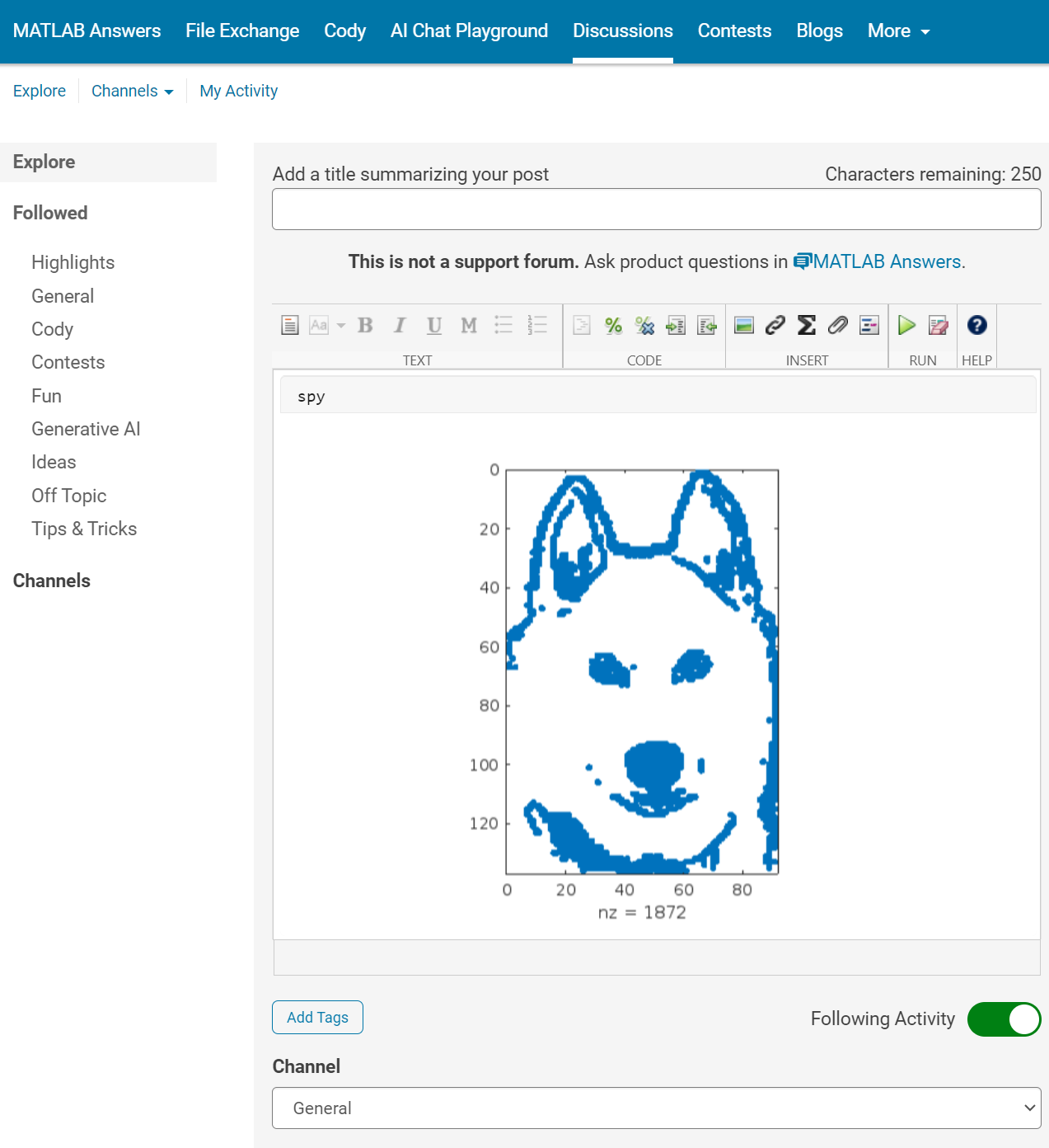
We're thrilled to share an exciting update with our community: the 'Run Code' feature is now available in the Discussions area!
Simply insert your code into the editor and press the green triangle button to run it. Your code will execute using the latest MATLAB R24a version, and it supports most common toolboxes. Moreover, this innovative feature allows for the running of attached files, further enhancing its utility and flexibility.
The ‘run code’ feature was first introduced in MATLAB Answers. Encouraged by the positive feedback and at the request of our community members, we are now expanding the availability of this feature to more areas within our community.
As always, your feedback is crucial to us, so please don't hesitate to share your thoughts and experiences by leaving a comment.