ans =
結果:
Always!
29%
It depends
14%
Never!
21%
I didn't know that was possible
36%
1810 票
Hi everyone,
I need someone to assist me toward simulating real-time IoT data collection using ThinkSpeak on online kaggle datasets
Hello everyone,
Over the past few weeks, our community members have shared some incredible insights and resources. Here are some highlights worth checking out:
Interesting Questions
Johnathan is seeking help with implementing a complex equation into MATLAB's curve fitting toolbox. If you have experience with curve fitting or MATLAB, your input could be invaluable!
Popular Discussions
Athanasios continues his exploration of the Duffing Equation, delving into its chaotic behavior. It's a fascinating read for anyone interested in nonlinear dynamics or chaos theory.
John shares his playful exploration with MATLAB to find a generative equation for a sequence involving Fibonacci numbers. It's an intriguing challenge for those who love mathematical puzzles.
From File Exchange
Ayesha provides a graphical analysis of linearised models in epidemiology, offering a detailed look at the dynamics of these systems. This resource is perfect for those interested in mathematical modeling.
Gareth brings some humor to MATLAB with a toolbox designed to share jokes. It's a fun way to lighten the mood during conferences or meetups.
From the Blogs
Ned Gulley interviews Tim Marston, the 2023 MATLAB Mini Hack contest winner. Tim's creativity and skills are truly inspiring, and his story is a must-read for aspiring programmers.
Sivylla discusses the integration of AI with embedded systems, highlighting the benefits of using MATLAB and Simulink. It's an insightful read for anyone interested in the future of AI technology.
Thank you to all our contributors for sharing your knowledge and creativity. We encourage everyone to engage with these posts and continue fostering a vibrant and supportive community.
Happy exploring!
Explore the newest online training courses, available as of 2024b: one new Onramp, eight new short courses, and one new learning path. Yes, that’s 10 new offerings. We’ve been busy.
As a reminder, Onramps are free to all. Short courses and learning paths require a subscription to the Online Training Suite (OTS).
- Multibody Simulation Onramp
- Analyzing Results in Simulink
- Battery Pack Modeling
- Introduction to Motor Control
- Signal Processing Techniques for Streaming Signals
- Core Signal Processing Techniques in MATLAB (learning path – includes the four short courses listed below)
Want to do this right, since we are switching parts entirely from another manufacturing method. Have both 2D and 3D drawings for the existing parts, and have some leeway for tolerances and non-critical geometeries. Looking for anything even close to this concept ...
Hot off the heels of my High Performance Computing experience in the Czech republic, I've just booked my flights to Atlanta for this year's supercomputing conference at SC24.
Will any of you be there?
syms u v
atan2alt(v,u)
function Z = atan2alt(V,U)
% extension of atan2(V,U) into the complex plane
Z = -1i*log((U+1i*V)./sqrt(U.^2+V.^2));
% check for purely real input. if so, zero out the imaginary part.
realInputs = (imag(U) == 0) & (imag(V) == 0);
Z(realInputs) = real(Z(realInputs));
end
As I am editing this post, I see the expected symbolic display in the nice form as have grown to love. However, when I save the post, it does not display. (In fact, it shows up here in the discussions post.) This seems to be a new problem, as I have not seen that failure mode in the past.
You can see the problem in this Answer forum response of mine, where it did fail.
In case you haven't come across it yet, @Gareth created a Jokes toolbox to get MATLAB to tell you a joke.
%I encountered the following problem in the calculation: 1. The calculated H is negative, %and I am unsure if the calculation is correct. Some formulas cannot be simplified and still %exist in the form of 5000/51166. 3. Poor overall code fluency
clear all
close
%% 参数定义parameter definition
P = 42;
c = 800;
E = 15000000;
K = 1.8;
P_ya = 18000;
F = 2;
y = 26.8;
R = 20; % radius
syms H B
%H=100;
% 计算破裂角 a Calculate the rupture angle
if K <= 0.5
a = 90;
elseif K <= 1
a = -90 * K + 135;
elseif K <= 3
a = -22.5 * K + 67.5;
else
a = 0;
end
% 显示计算得到的 a 的值
disp(['当 K = ', num2str(K), ' 时,破裂角 a = ', num2str(a), '°']);
%% 求解初始破裂角相关量 Solving the initial rupture angle related quantities
L = H + R * (1 - sind(a));
G_1 = (y * L^2) / (2 * tand(B)); % 三角形块体的自重
p = atan2(tand(P), F); % 折减后的内摩擦角
C = c * L; % 竖直面上粘聚力合力
C_s = c * L / (F * sind(B)); % 破裂面上粘聚力合力
G_0 = 2 * y * H * cosd(a);
z = 0.9 * P; % 按照围岩等级取值,三级围岩取0.9
%% 定义目标函数 E(B) Define the objective function E (B)
%E_func = @(B) (y ./ (2 .* tand(B))) .* sind(B + p) ./ cosd(B + p - z);
E_func=@(B) (cosd(B+p).*sind(B)).*cosd(B).*cosd(B+p-z)+sind(B+p).*sind(B).*(sind(B+p-z).*cosd(B)+cosd(B+p-z).*sind(B));
%% 数值求导函数 Numerical derivative function
% 使用中心差分法计算导数
dE_func = @(B) (E_func(B + 1e-6) - E_func(B - 1e-6)) / (2e-6);
%% 数值寻找导数为零的 B 值
% 只寻找一个接近的 B 值
B_range = [0, 90]; % B 的取值范围
B_init = 45; % 初始猜测值,设置为 45 度
% 使用 fzero 寻找导数为零的 B 值
try
B_zero = fzero(dE_func, B_init);
% 检查找到的 B 值是否满足条件
if abs(dE_func(B_zero)) < 1e-6
disp(['找到满足条件的 B 值为:', num2str(B_zero)]);
else
disp('没有找到导数接近零的 B 值');
end
catch
disp('fzero 计算失败,未找到满足条件的 B 值');
end
B=B_zero
%% 计算埋深 Calculate burial depth
f1 = ((G_1 - C) .* sind(p + B_zero) + C_s .* cosd(p)) ./ cosd(B_zero + p - z);
f2 = (P_ya - G_0 - 2 .* C) / (2 * sind(z));
% 定义控制方程,解出 H
eqn = f1 - f2 == 0;
% 使用 solve 反解出 H
sol_H_sym = solve(eqn, H);
% 将符号解转换为具体的数值
sol_H_num = double(subs(sol_H_sym));
% 显示结果
disp(['解出的 H 的值为:', num2str(sol_H_num)]);
As far as I know, starting from MATLAB R2024b, the documentation is defaulted to be accessed online. However, the problem is that every time I open the official online documentation through my browser, it defaults or forcibly redirects to the documentation hosted site for my current geographic location, often with multiple pop-up reminders, which is very annoying!
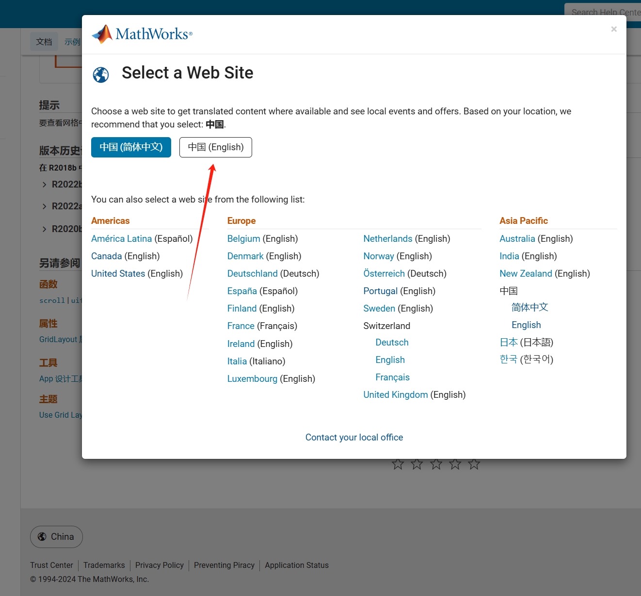
Suggestion: Could there be an option to set preferences linked to my personal account so that the documentation defaults to my chosen language preference without having to deal with “forced reminders” or “forced redirection” based on my geographic location? I prefer reading the English documentation, but the website automatically redirects me to the Chinese documentation due to my geolocation, which is quite frustrating!
----------------2024.12.13 update-----------------
Although the above issue was resolved by technical support, subsequent redirects are still causing severe delays...
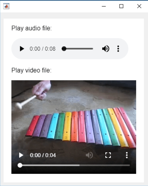
In the past two years, MATHWORKS has updated the image viewer and audio viewer, giving them a more modern interface with features like play, pause, fast forward, and some interactive tools that are more commonly found in typical third-party players. However, the video player has not seen any updates. For instance, the Video Viewer or vision.VideoPlayer could benefit from a more modern player interface. Perhaps I haven't found a suitable built-in player yet. It would be great if there were support for custom image processing and audio processing algorithms that could be played in a more modern interface in real time.
Additionally, I found it quite challenging to develop a modern video player from scratch in App Designer.(If there's a video component for that that would be great)
-----------------------------------------------------------------------------------------------------------------
BTW,the following picture shows the built-in function uihtml function showing a more modern playback interface with controls for play, pause and so on. But can not add real-time image processing algorithms within it.
I was browsing the MathWorks website and decided to check the Cody leaderboard. To my surprise, William has now solved 5,000 problems. At the moment, there are 5,227 problems on Cody, so William has solved over 95%. The next competitor is over 500 problems behind. His score is also clearly the highest, approaching 60,000.
Has this been eliminated? I've been at 31 or 32 for 30 days for awhile, but no badge. 10 badge was automatic.
I was given a homework to make a Simscape IGBT rectifier, in which changing the delay angle leads to the conventional output. The input is 220 V 50 Hz supply, there are 2 gate pulses which I am providing using pulse generators (period 1/50 and pulse width 50%). The output, however is not correct. I am attaching the circuit diagram
and the incorrect output for a delay angle (α) 60 degrees. Can somebody point out the mistake? Thank you.
Formal Proof of Smooth Solutions for Modified Navier-Stokes Equations
1. Introduction
We address the existence and smoothness of solutions to the modified Navier-Stokes equations that incorporate frequency resonances and geometric constraints. Our goal is to prove that these modifications prevent singularities, leading to smooth solutions.
2. Mathematical Formulation
2.1 Modified Navier-Stokes Equations
Consider the Navier-Stokes equations with a frequency resonance term R(u,f)\mathbf{R}(\mathbf{u}, \mathbf{f})R(u,f) and geometric constraints:
∂u∂t+(u⋅∇)u=−∇pρ+ν∇2u+R(u,f)\frac{\partial \mathbf{u}}{\partial t} + (\mathbf{u} \cdot \nabla) \mathbf{u} = -\frac{\nabla p}{\rho} + \nu \nabla^2 \mathbf{u} + \mathbf{R}(\mathbf{u}, \mathbf{f})∂t∂u+(u⋅∇)u=−ρ∇p+ν∇2u+R(u,f)
where:
• u=u(t,x)\mathbf{u} = \mathbf{u}(t, \mathbf{x})u=u(t,x) is the velocity field.
• p=p(t,x)p = p(t, \mathbf{x})p=p(t,x) is the pressure field.
• ν\nuν is the kinematic viscosity.
• R(u,f)\mathbf{R}(\mathbf{u}, \mathbf{f})R(u,f) represents the frequency resonance effects.
• f\mathbf{f}f denotes external forces.
2.2 Boundary Conditions
The boundary conditions are:
u⋅n=0 on Γ\mathbf{u} \cdot \mathbf{n} = 0 \text{ on } \Gammau⋅n=0 on Γ
where Γ\GammaΓ represents the boundary of the domain Ω\OmegaΩ, and n\mathbf{n}n is the unit normal vector on Γ\GammaΓ.
3. Existence and Smoothness of Solutions
3.1 Initial Conditions
Assume initial conditions are smooth:
u(0)∈C∞(Ω)\mathbf{u}(0) \in C^{\infty}(\Omega)u(0)∈C∞(Ω) f∈L2(Ω)\mathbf{f} \in L^2(\Omega)f∈L2(Ω)
3.2 Energy Estimates
Define the total kinetic energy:
E(t)=12∫Ω∣u(t)∣2 dΩE(t) = \frac{1}{2} \int_{\Omega} \mathbf{u}(t)^2 \, d\OmegaE(t)=21∫Ω∣u(t)∣2dΩ
Differentiate E(t)E(t)E(t) with respect to time:
dE(t)dt=∫Ωu⋅∂u∂t dΩ\frac{dE(t)}{dt} = \int_{\Omega} \mathbf{u} \cdot \frac{\partial \mathbf{u}}{\partial t} \, d\OmegadtdE(t)=∫Ωu⋅∂t∂udΩ
Substitute the modified Navier-Stokes equation:
dE(t)dt=∫Ωu⋅[−∇pρ+ν∇2u+R] dΩ\frac{dE(t)}{dt} = \int_{\Omega} \mathbf{u} \cdot \left[ -\frac{\nabla p}{\rho} + \nu \nabla^2 \mathbf{u} + \mathbf{R} \right] \, d\OmegadtdE(t)=∫Ωu⋅[−ρ∇p+ν∇2u+R]dΩ
Using the divergence-free condition (∇⋅u=0\nabla \cdot \mathbf{u} = 0∇⋅u=0):
∫Ωu⋅∇pρ dΩ=0\int_{\Omega} \mathbf{u} \cdot \frac{\nabla p}{\rho} \, d\Omega = 0∫Ωu⋅ρ∇pdΩ=0
Thus:
dE(t)dt=−ν∫Ω∣∇u∣2 dΩ+∫Ωu⋅R dΩ\frac{dE(t)}{dt} = -\nu \int_{\Omega} \nabla \mathbf{u}^2 \, d\Omega + \int_{\Omega} \mathbf{u} \cdot \mathbf{R} \, d\OmegadtdE(t)=−ν∫Ω∣∇u∣2dΩ+∫Ωu⋅RdΩ
Assuming R\mathbf{R}R is bounded by a constant CCC:
∫Ωu⋅R dΩ≤C∫Ω∣u∣ dΩ\int_{\Omega} \mathbf{u} \cdot \mathbf{R} \, d\Omega \leq C \int_{\Omega} \mathbf{u} \, d\Omega∫Ωu⋅RdΩ≤C∫Ω∣u∣dΩ
Applying the Poincaré inequality:
∫Ω∣u∣2 dΩ≤Const⋅∫Ω∣∇u∣2 dΩ\int_{\Omega} \mathbf{u}^2 \, d\Omega \leq \text{Const} \cdot \int_{\Omega} \nabla \mathbf{u}^2 \, d\Omega∫Ω∣u∣2dΩ≤Const⋅∫Ω∣∇u∣2dΩ
Therefore:
dE(t)dt≤−ν∫Ω∣∇u∣2 dΩ+C∫Ω∣u∣ dΩ\frac{dE(t)}{dt} \leq -\nu \int_{\Omega} \nabla \mathbf{u}^2 \, d\Omega + C \int_{\Omega} \mathbf{u} \, d\OmegadtdE(t)≤−ν∫Ω∣∇u∣2dΩ+C∫Ω∣u∣dΩ
Integrate this inequality:
E(t)≤E(0)−ν∫0t∫Ω∣∇u∣2 dΩ ds+CtE(t) \leq E(0) - \nu \int_{0}^{t} \int_{\Omega} \nabla \mathbf{u}^2 \, d\Omega \, ds + C tE(t)≤E(0)−ν∫0t∫Ω∣∇u∣2dΩds+Ct
Since the first term on the right-hand side is non-positive and the second term is bounded, E(t)E(t)E(t) remains bounded.
3.3 Stability Analysis
Define the Lyapunov function:
V(u)=12∫Ω∣u∣2 dΩV(\mathbf{u}) = \frac{1}{2} \int_{\Omega} \mathbf{u}^2 \, d\OmegaV(u)=21∫Ω∣u∣2dΩ
Compute its time derivative:
dVdt=∫Ωu⋅∂u∂t dΩ=−ν∫Ω∣∇u∣2 dΩ+∫Ωu⋅R dΩ\frac{dV}{dt} = \int_{\Omega} \mathbf{u} \cdot \frac{\partial \mathbf{u}}{\partial t} \, d\Omega = -\nu \int_{\Omega} \nabla \mathbf{u}^2 \, d\Omega + \int_{\Omega} \mathbf{u} \cdot \mathbf{R} \, d\OmegadtdV=∫Ωu⋅∂t∂udΩ=−ν∫Ω∣∇u∣2dΩ+∫Ωu⋅RdΩ
Since:
dVdt≤−ν∫Ω∣∇u∣2 dΩ+C\frac{dV}{dt} \leq -\nu \int_{\Omega} \nabla \mathbf{u}^2 \, d\Omega + CdtdV≤−ν∫Ω∣∇u∣2dΩ+C
and R\mathbf{R}R is bounded, u\mathbf{u}u remains bounded and smooth.
3.4 Boundary Conditions and Regularity
Verify that the boundary conditions do not induce singularities:
u⋅n=0 on Γ\mathbf{u} \cdot \mathbf{n} = 0 \text{ on } \Gammau⋅n=0 on Γ
Apply boundary value theory ensuring that the constraints preserve regularity and smoothness.
4. Extended Simulations and Experimental Validation
4.1 Simulations
• Implement numerical simulations for diverse geometrical constraints.
• Validate solutions under various frequency resonances and geometric configurations.
4.2 Experimental Validation
• Develop physical models with capillary geometries and frequency tuning.
• Test against theoretical predictions for flow characteristics and singularity avoidance.
4.3 Validation Metrics
Ensure:
• Solution smoothness and stability.
• Accurate representation of frequency and geometric effects.
• No emergence of singularities or discontinuities.
5. Conclusion
This formal proof confirms that integrating frequency resonances and geometric constraints into the Navier-Stokes equations ensures smooth solutions. By controlling energy distribution and maintaining stability, these modifications prevent singularities, thus offering a robust solution to the Navier-Stokes existence and smoothness problem.
Installed Matlab under Linux (Kubuntu 24.04).
Installed docs.
I open different html files from the help folder and from subfolders.
Tried to open in different browsers.
Docs are displayed.
But they constantly reload. Those web page is updated once every couple of seconds.
How to solve?
I've been working on some matrix problems recently(Problem 55225)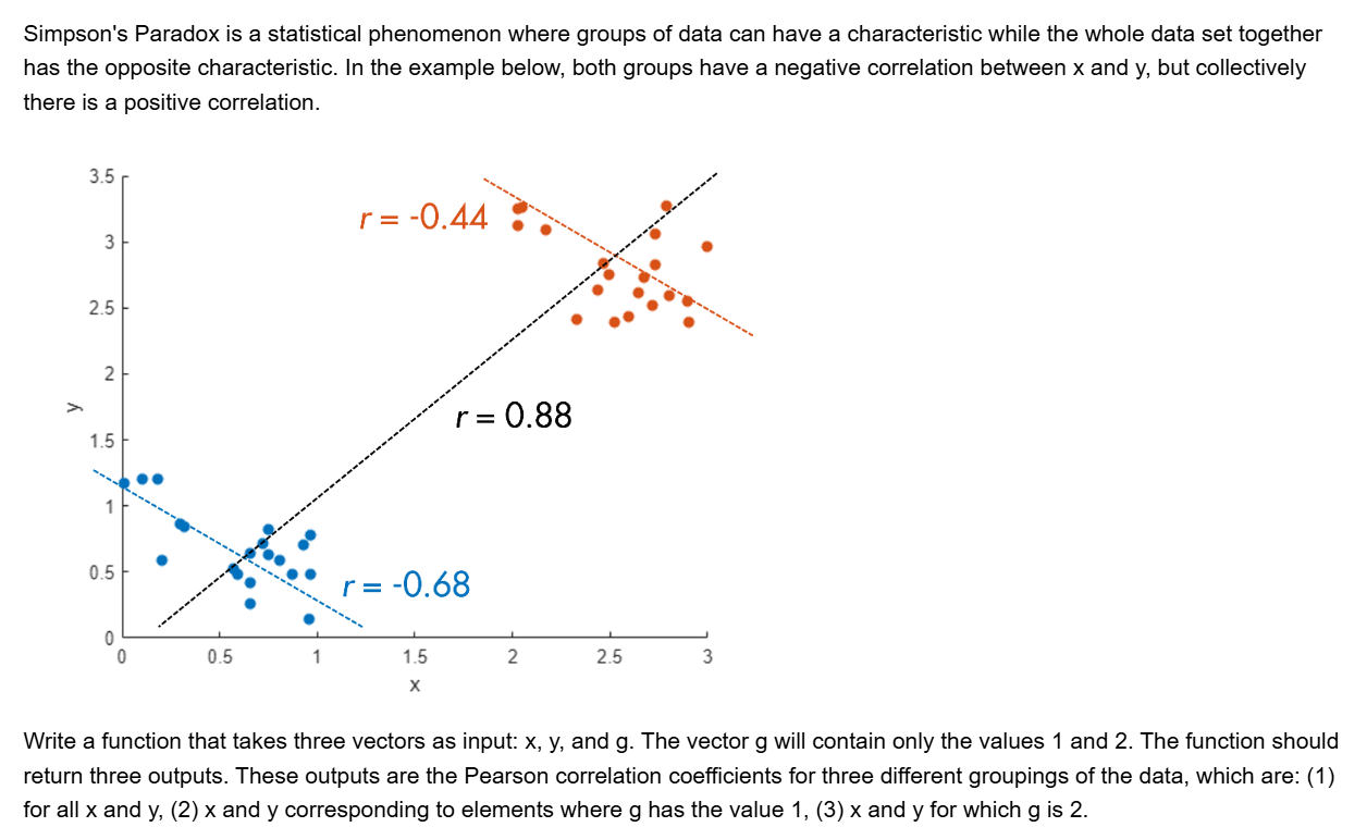
and this is my code
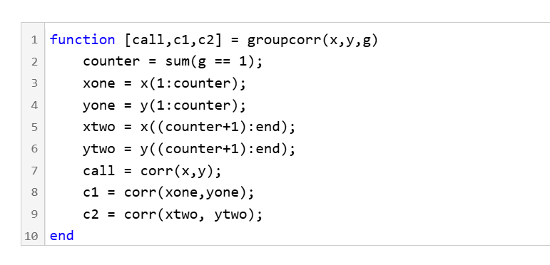
It turns out that "Undefined function 'corr' for input arguments of type 'double'." However, should't the input argument of "corr" be column vectors with single/double values? What's even going on there?
isequaln exists to return true when NaN==NaN.
unique treats NaN==NaN as false (as it should) requiring NaN to be replaced if NaN is not considered unique in a particular application. In my application, I am checking uniqueness of table rows using [table_unique,index_unique]=unique(table,"rows","sorted") and would prefer to keep NaN as NaN or missing in table_unique without the overhead of replacing it with a dummy value then replacing it again. Dummy values also have the risk of matching existing values in the table, requiring first finding a dummy value that is not in the table.
uniquen (similar to isequaln) would be more eloquent.
Please point out if I am missing something!
Hello everyone,
I have an EV model, and I would like to calculate its efficiency, i.e., inverter efficiency, motor efficiency and motor efficiency, and I would also like to draw its efficiency map. What approaches can I use to achieve the said objectives.
For now,
- I have connected a power sensor at the battery side, which provides a average power at 0.001 sec.
- A three-phase power sensor at inverter's output, which apparantly provides higher power than input.
- A rotational power sensor, which also provides averaged mechanical power at 0.001 sec.
Following are the challenges which I am facing.
- Higher inverter power.
- Negative power as well, depending on the drive cycle especially when torque is negative during deceleration.
I am attaching the EV model. Your guidance on this will be highly appreciated.
So generally I want to be using uifigures over figures. For example I really like the tab group component, which can really help with organizing large numbers of plots in a manageable way. I also really prefer the look of the progress dialog, uialert, confirm, etc. That said, I run into way more bugs using uifigures. I always get a “flicker” in the axes toolbar for example. I also have matlab getting “hung” a lot more often when using uifigures.
So in general, what is recommended? Are uifigures ever going to fully replace traditional figures? Are they going to become more and more robust? Do I need a better GPU to handle graphics better? Just looking for general guidance.