filterbank

Wavelet and scaling filters

Syntax

phif = filterbank(sf)

[phif,psifilters] = filterbank(sf)

[phif,psifilters,f] = filterbank(sf)

[phif,psifilters,f,filterparams] = filterbank(sf)

[___] = filterbank(sf,fb)

Description

phif = filterbank(sf) returns the Fourier transform of the scaling filter for the 2-D wavelet scattering network, sf. phif is a single or double-precision matrix depending on the value of the Precision property of the scattering network. phif has dimensions M-by-N, where M and N are the padded row and column sizes of the scattering network.

[phif,psifilters] = filterbank(sf) returns the Fourier transforms for the wavelet filters in psifilters. psifilters is an Nfb-by-1 cell array, where Nfb is the number of filter banks in the scattering network. Each element of psifilters is a 3-D array. The 3-D arrays are M-by-N-by-L, where M and N are the padded row and column sizes of the wavelet filters and L is the number of wavelet filters for each filter bank. The wavelet filters are ordered by increasing scale with NumRotations wavelet filters for each scale. Within a scale, the wavelet filters are ordered by rotation angle.

[phif,psifilters,f] = filterbank(sf) returns the center spatial frequencies for the wavelet filters in psifilters. f is an Nfb-by-1 cell array, where Nfb is the number of filter banks in sf. The jth element of f contains the center frequencies for the jth wavelet filter bank in psifilters. Each element of f is a L-by-2 matrix with each row containing the center frequencies of the corresponding Lth wavelet.

[phif,psifilters,f,filterparams] = filterbank(sf) returns the filter parameters for the 2-D scattering network. filterparams is an Nfb-by-1 cell array of MATLAB^® tables, where the jth element of filterparams is a MATLAB table containing the filter parameters for the jth filter bank

[___] = filterbank(sf,fb) returns the desired outputs for the filter banks specified in fb. fb is a scalar or vector of integers between 1 and numfilterbanks(sf) inclusive. If fb is a scalar, psifilters is an M-by-N-by-L matrix, and filterparams is a MATLAB table.

Examples

Plot Wavelet Center Frequencies

This example shows how to plot the scaling filter and the wavelet filter center frequencies for a two-filter bank wavelet image scattering network.

Create a wavelet image scattering network with two filter banks. The first filter bank has a quality factor of 2, and the second filter bank has a quality factor of 1.

sf = waveletScattering2(QualityFactors=[2 1])

sf = 
  waveletScattering2 with properties:

             ImageSize: [128 128]
       InvarianceScale: 64
          NumRotations: [6 6]
        QualityFactors: [2 1]
             Precision: 'single'
    OversamplingFactor: 0
          OptimizePath: 1

Obtain the scaling filter, wavelet filters, and wavelet center frequencies for the network.

[phif,psifilters,f] = filterbank(sf);

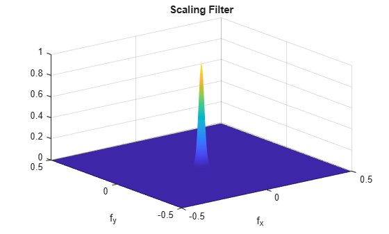
Make a surface plot of the scaling filter.

Nx = size(phif,1);
Ny = size(phif,2);
fx = -1/2:1/Nx:1/2-1/Nx;
fy = -1/2:1/Ny:1/2-1/Ny;
surf(fx,fy,fftshift(phif))
shading interp
title("Scaling Filter")
xlabel("f_x")
ylabel("f_y")

Plot the wavelet center frequencies for the two filter banks.

plot(f{1}(:,1),f{1}(:,2),"k*")
hold on
plot(f{2}(:,1),f{2}(:,2),"r^",MarkerFaceColor=[1 0 0])
hold off
grid on
axis equal
xlabel("f_x")
ylabel("f_y")
legend("First Filter Bank Q = 2","Second Filter Bank Q = 1")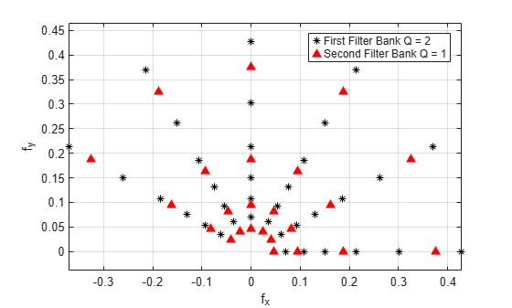

Plot Specific Wavelet of Image Scattering Network

This example shows how to obtain and plot a specific wavelet of a wavelet image scattering network.

Create a wavelet image scattering network with two filter banks. The first filter bank has a quality factor of 2 and seven rotations per wavelet. The second filter bank has a quality factor of 1 and five rotations per wavelet.

sf = waveletScattering2(QualityFactors=[2 1],NumRotations=[7 5])

sf = 
  waveletScattering2 with properties:

             ImageSize: [128 128]
       InvarianceScale: 64
          NumRotations: [7 5]
        QualityFactors: [2 1]
             Precision: 'single'
    OversamplingFactor: 0
          OptimizePath: 1

Obtain the wavelet filters and center frequencies for the network. Return the dimensions of the two cell arrays.

[~,psifilters,f] = filterbank(sf);
psifilters

psifilters=2×1 cell array
    {192×192×42 single}
    {192×192×20 single}

f

f=2×1 cell array
    {42×2 double}
    {20×2 double}

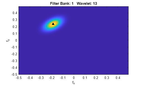
The first filter bank has 42 wavelet filters, and the second filter bank has 20 filters. The number of filters in each filter bank is a multiple of the corresponding value in NumRotations. Use the helper function helperPlotWavelet to plot a specific wavelet and mark its center frequency.

whichFilterBank = 1;
whichWavelet = 13;
helperPlotWavelet(psifilters,f,whichFilterBank,whichWavelet)

Appendix

The following helper function is used in this example.

function helperPlotWavelet(psiFilters,psiFreq,filBank,wvFilter)
Nx = size(psiFilters{filBank},2);
Ny = size(psiFilters{filBank},1);
fx = -1/2:1/Nx:1/2-1/Nx;
fy = -1/2:1/Ny:1/2-1/Ny;
imagesc(fx,fy,fftshift(psiFilters{filBank}(:,:,wvFilter)))
hold on
plot(psiFreq{filBank}(wvFilter,1),psiFreq{filBank}(wvFilter,2),...
    "k^",MarkerFaceColor=[0 0 0])
hold off
axis xy
xlabel("f_x")
ylabel("f_y")
str = sprintf("Filter Bank: %d   Wavelet: %d",filBank,wvFilter);
title(str)
end

Determine Wavelet Semi-Major Axis

This example shows how to determine the semi-major axis of a wavelet filter in a 2-D wavelet scattering network.

Create a 2-D wavelet scattering network. The network has two filter banks with quality factors of 2 and 1, respectively. There are seven rotations per wavelet in the first filter bank and five rotations per wavelet in the second filter bank. Return the Fourier transforms of the wavelet filters and their center spatial frequencies, and the filter bank parameters.

sf = waveletScattering2(QualityFactors=[2 1],NumRotations=[7 5]);
[~,psif,f,fparams] = filterbank(sf);

The wavelet filters in psif are ordered by increasing scale, with NumRotations wavelet filters for each scale. Within a scale, the wavelet filters are ordered by rotation.

Return the reported 3 dB bandwidths, rotation angles, and slant parameter of the first filter bank. Return the dimensions of the matrix containing the wavelet filters of the first filter bank. Confirm that (number of rotations) $\times$ (number of bandwidths) equals the size of the third dimension of the matrix. The product is the number of wavelet filters in the filter bank. The row and column sizes are the dimensions of the padded wavelet filters. Note that the slant parameter is less than 1.

fparams{1}.psi3dBbw

ans = 1×6

    0.1464    0.1036    0.0732    0.0518    0.0366    0.0366

fparams{1}.rotations

ans = 1×7

         0    0.4488    0.8976    1.3464    1.7952    2.2440    2.6928

fparams{1}.slant

ans = 
0.5817

size(psif{1})

ans = 1×3

   192   192    42

The vector fparams{1}.psi3dBbw has six elements. The number of elements is equal to the number of wavelet scales in the first filter bank.

From the first filter bank, obtain the unrotated wavelet filter from the second finest scale. Obtain the center spatial frequency of the wavelet. Use the helper function helperPlotWaveletFT to plot the wavelet and mark its center frequency. The code for helperPlotWaveletFT is shown at the end of this example.

whichFilterBank = 1;
whichScale = 2;
whichRotAngle = 1;
numRot = sf.NumRotations(whichFilterBank);

wvf = psif{whichFilterBank}(:,:,1+(whichScale-1)*numRot+(whichRotAngle-1));
wvfCenFrq = f{whichFilterBank}(1+(whichScale-1)*numRot+(whichRotAngle-1),:);

helperPlotWaveletFT(wvf,wvfCenFrq)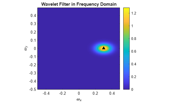

Take the inverse Fourier transform of the wavelet filter. The filter is strictly real, and the inverse Fourier transform is complex-valued. Use the helper function helperPlotWavelet to plot the absolute value of the wavelet. The code for helperPlotWavelet is shown at the end of this example.

wvf_ifft = ifft2(wvf);
helperPlotWavelet(wvf_ifft)

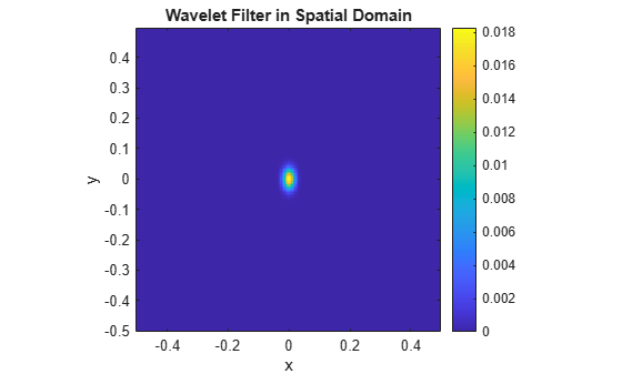
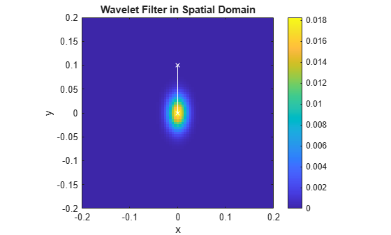
Note that the semi-major axis of the wavelet support is in the y-direction. This is consistent with a slant parameter whose value is less than 1. The vector (0,0.1) coincides with the semi-major axis. Plot the vector in the previous figure.

vec = [0 0.1];
hold on
plot([0 vec(1)],[0 vec(2)],"wx-")
hold off
xlim([-0.2 0.2])
ylim([-0.2 0.2])

From the same filter bank and scale, choose a rotated wavelet filter. Plot the absolute value of the wavelet in the spatial domain. Use the associated rotation angle in fparams{1}.rotations, and rotate clockwise the vector (0,0.1) by that amount. Plot the rotated vector in the figure. Confirm that the vector is aligned with the semi-major axis of the rotated wavelet.

whichRotAngle = 3;
rotAngle = fparams{whichFilterBank}.rotations(whichRotAngle);
rmat = [cos(rotAngle) sin(rotAngle) ; -sin(rotAngle) cos(rotAngle)];

wvf = psif{whichFilterBank}(:,:,1+(whichScale-1)*numRot+(whichRotAngle-1));
wvf_ifft = ifft2(wvf);

rvec = rmat*vec'; 

helperPlotWavelet(wvf_ifft)
hold on
plot([0 rvec(1)],[0 rvec(2)],"wx-")
xlim([-0.2 0.2])
ylim([-0.2 0.2])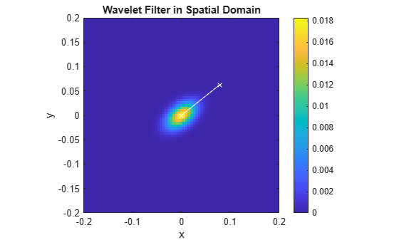

Appendix

The following helper functions are used in this example.

helperPlotWaveletFT — Plot in the frequency domain

function helperPlotWaveletFT(wavelet,cenFreq)
Nx = size(wavelet,2);
Ny = size(wavelet,1);
fx = -1/2:1/Nx:1/2-1/Nx;
fy = -1/2:1/Ny:1/2-1/Ny;
imagesc(fx,fy,fftshift(wavelet))
colorbar
hold on
plot(cenFreq(1),cenFreq(2),"k^",MarkerFaceColor=[0 0 0])
hold off
xlabel("$\omega_x$",Interpreter="latex")
ylabel("$\omega_y$",Interpreter="latex")
axis xy
axis equal
axis tight
title("Wavelet Filter in Frequency Domain")
end

helperPlotWavelet — Plot in the spatial domain

function helperPlotWavelet(wavelet)
Nx = size(wavelet,2);
Ny = size(wavelet,1);
fx = -1/2:1/Nx:1/2-1/Nx;
fy = -1/2:1/Ny:1/2-1/Ny;
imagesc(fx,fy,abs(fftshift(wavelet)))
colorbar
axis xy
xlabel("x")
ylabel("y")
axis equal
axis tight
title('Wavelet Filter in Spatial Domain')
end

Input Arguments

sf — Wavelet image scattering network

waveletScattering2 object

Wavelet image scattering network, specified as a waveletScattering2 object.

fb — Filter banks

positive integer | vector of positive integers

Filter banks, specified as an integer or vector of integers between 1 and numfilterbanks(sf) inclusive. If fb is a scalar, psifilters is an M-by-N-by-L matrix and filterparams is a MATLAB table.

Output Arguments

phif — Fourier transform of scaling filter

real-valued matrix

Fourier transform of scaling filter, returned as a real-valued 2-D matrix. The precision of phif depends on the value of the Precision property of the scattering network. phif has dimensions M-by-N, where M and N are the padded row and column sizes of the scattering network.

psifilters — Fourier transforms of the wavelet filters

cell array

Fourier transforms of the wavelet filters, returned as an Nfb-by-1 cell array, where Nfb is the number of filter banks in the scattering network. Each element of psifilters is a 3-D array. The 3-D arrays are M-by-N-by-L, where M and N are the padded row and column sizes of the wavelet filters and L is the number of wavelet filters for each filter bank. The wavelet filters are ordered by increasing scale with NumRotations wavelet filters for each scale.

Example: Note that size(psifilters,3) is equal to size(f,1).

f — Center spatial frequencies

cell array

Center spatial frequencies of the wavelet filters, returned as a Nfb-by-1 cell array where Nfb is the number of filter banks in the scattering network. The jth element of f contains the center frequencies for the jth wavelet filter bank in psifilters. Each element of f is an L-by-2 matrix with each row containing the center frequencies of the corresponding Lth wavelet. The spatial frequencies are in cycles per pixel.

filterparams — Filter parameters

cell array

Filter parameters for the 2-D scattering network, sf. filterparams is an Nfb-by-1 cell array of MATLAB tables, where the jth element of filterparams is a MATLAB table containing the filter parameters for the jth filter bank. Each table contains these variables:

• Q — The quality factor of the filter bank, returned as an integer.

• J — The highest factor used in the dilation of the Morlet wavelets, 2^J/Q, returned as an integer.

• precision — The precision of the scattering network, returned as 'single' or 'double'.

• omegapsi — The wavelet center frequencies in descending order (highest to lowest), returned as a vector.

• freqsigmapsi — The wavelet frequency standard deviations, returned as a vector.

• slant — The slant parameter for the spatial vertical semi-major axis of the wavelet, returned as a real number. The slant parameter, also known as the spatial aspect ratio, characterizes the shape of the support of the wavelet.

• spatialsigmapsi — The wavelet spatial standard deviations, returned as a vector.

• spatialsigmaphi — The scaling filter spatial standard deviation, returned as a real number.

• psi3dBbw — The wavelet 3 dB bandwidths, returned as a vector.

• psiftsupport — The wavelet frequency support, returned as a vector.

• phiftsupport — The scaling filter frequency support, returned as a real number.

• phi3dBbw — The scaling filter 3 dB bandwidth, returned as a real number.

• rotations — The wavelet orientation angles in radians, returned as a vector. The length of rotations equals the NumRotations value associated with the filter bank.

The following vectors in the table have equal length: omegapsi, freqsigmapsi, spatialsigmapsi, psi3dBbw, and psiftsupport.

The total number of wavelet filters in a filter bank is length(omegapsi)×length(rotations). See Determine Wavelet Semi-Major Axis.

More About

Slant Parameter

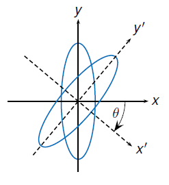
The slant parameter or spatial aspect ratio controls the shape of the elliptical support of the Morlet wavelet.

The Morlet wavelet is of the form

$$\psi (x,y)=e^{-(x^2+{\nu }^2{y}^2)/2{\sigma }^2}{e}^{i{\omega }_{\lambda }x}$$

where v is the slant parameter. Typically, v < 1, so that the ellipse $$\begin{array}{l}\frac{x^2}{{\sigma }^2}+\frac{y^2}{{\sigma }^2/{\nu }^2}\\ \end{array}$$ is elongated spatially in the y-direction. The wavelet is rotated in a clockwise direction: $$\left(\begin{array}{c}x\prime \\ y\prime \end{array}\right)=\left(\begin{array}{cc}\cos \theta & \sin \theta \\ -\sin \theta & \cos \theta \end{array}\right)\left(\begin{array}{c}x\\ y\end{array}\right)$$.

The rotated Morlet wavelet is of the form

$$\psi (x^{\prime },y\text{'})=e^{-({x^{\prime }}^2+{\nu }^2{y^{\prime }}^2)/2{\sigma }^2}{e}^{i{\omega }_{\lambda }{x}^{\prime }}$$

If g(x,y) and G(ω_x,ω_y) form a Fourier pair: $$g(x,y)\stackrel{FT}{\leftrightarrow }G({\omega }_x,{\omega }_y)$$, then so do their rotations:

$$g(x\cos \theta +y\sin \theta ,-x\sin \theta +y\cos \theta )\stackrel{FT}{\leftrightarrow }G({\omega }_x\cos \theta +{\omega }_y\sin \theta ,-{\omega }_x\sin \theta +{\omega }_y\cos \theta )$$

The Fourier transform of the Morlet wavelet is

$$\widehat{\psi }({\omega }_x,{\omega }_y)=\frac{2\pi {\sigma }^2}{\nu }{e}^{-\frac{{\sigma }^2}{\nu }\left({({\omega }_x-{\omega }_{\lambda })}^2+\frac{{\omega }_y}{{\nu }^2}\right)}$$

A given wavelet ψ(x,y) has a reported bandwidth bw. The reported bandwidth is dependent on the scale, but not the rotation angle. For a reported 3 dB bandwidth bw, the bandwidth along the semi-major spatial axis of the ellipse that describes the wavelet support is bw × slant.

The semi-major spatial axis depends on the rotation angle. The semi-major spatial axis can be computed from the vector rotations in the output argument filterparams.

As ordered in the output arguments f and psifilters, the wavelet filter psifilters(:,:,1 + k × NumRotations) for an integer k is the first, unrotated wavelet at a given scale. The wavelet has a center spatial frequency of f(1 + k × NumRotations,:), which is of the form (ωx,0). See Determine Wavelet Semi-Major Axis.

Version History

Introduced in R2019a