biorfilt
Biorthogonal wavelet filter set
Syntax
Description
[
returns four filters associated with the
biorthogonal wavelet specified by decomposition
filter LoD,HiD,LoR,HiR] = biorfilt(DF,RF)DF and reconstruction
filter RF. These filters are
LoD— Decomposition lowpass filterHiD— Decomposition highpass filterLoR— Reconstruction lowpass filterHiR— Reconstruction highpass filter
[
returns eight filters, the first four associated
with the decomposition wavelet, and the last four
associated with the reconstruction wavelet.LoD1,HiD1,LoR1,HiR1,LoD2,HiD2,LoR2,HiR2] = biorfilt(DF,RF,'8')
Examples
This example shows how to obtain the decomposition (analysis) and reconstruction (synthesis) filters for the 'bior3.5' wavelet.
Obtain the two scaling and wavelet filters associated with the 'bior3.5' wavelet.
wv = 'bior3.5';
[Rf,Df] = biorwavf(wv);
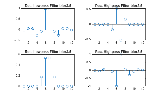
[LoD,HiD,LoR,HiR] = biorfilt(Df,Rf);Plot the filter impulse responses.
subplot(2,2,1)
stem(LoD)
title(['Dec. Lowpass Filter ',wv])
subplot(2,2,2)
stem(HiD)
title(['Dec. Highpass Filter ',wv])
subplot(2,2,3)
stem(LoR)
title(['Rec. Lowpass Filter ',wv])
subplot(2,2,4)
stem(HiR)
title(['Rec. Highpass Filter ',wv])
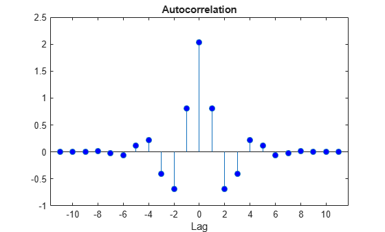
Demonstrate that autocorrelations at even lags are only zero for dual pairs of filters. Examine the autocorrelation sequence for the lowpass decomposition filter.
npad = 2*length(LoD)-1;
LoDxcr = fftshift(ifft(abs(fft(LoD,npad)).^2));
lags = -floor(npad/2):floor(npad/2);
figure
stem(lags,LoDxcr,'markerfacecolor',[0 0 1])
set(gca,'xtick',-10:2:10)
title('Autocorrelation')
xlabel('Lag')
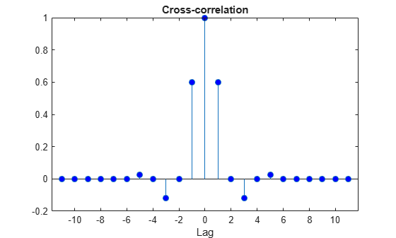
Examine the cross-correlation sequence for the lowpass decomposition and synthesis filters. Compare the result with the preceding figure. At even lags, the cross-correlation is zero.
npad = 2*length(LoD)-1;
xcr = fftshift(ifft(fft(LoD,npad).*conj(fft(LoR,npad))));
lags = -floor(npad/2):floor(npad/2);
stem(lags,xcr,'markerfacecolor',[0 0 1])
set(gca,'xtick',-10:2:10)
title('Cross-correlation')
xlabel('Lag')
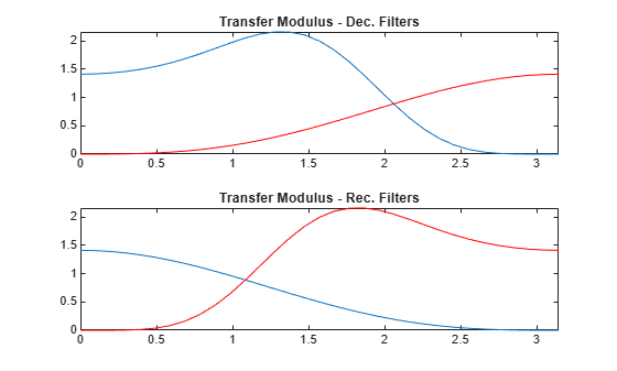
Compare the transfer functions of the analysis and synthesis scaling and wavelet filters.
dftLoD = fft(LoD,64);
dftLoD = dftLoD(1:length(dftLoD)/2+1);
dftHiD= fft(HiD,64);
dftHiD = dftHiD(1:length(dftHiD)/2+1);
dftLoR = fft(LoR,64);
dftLoR = dftLoR(1:length(dftLoR)/2+1);
dftHiR = fft(HiR,64);
dftHiR = dftHiR(1:length(dftHiR)/2+1);
df = (2*pi)/64;
freqvec = 0:df:pi;

subplot(2,1,1)
plot(freqvec,abs(dftLoD),freqvec,abs(dftHiD),'r')
axis tight
title('Transfer Modulus - Dec. Filters')
subplot(2,1,2)
plot(freqvec,abs(dftLoR),freqvec,abs(dftHiR),'r')
axis tight
title('Transfer Modulus - Rec. Filters')
Input Arguments
Output Arguments
More About
References
[1] Cohen, Albert. "Ondelettes, analyses multirésolution et traitement numérique du signal," Ph. D. Thesis, University of Paris IX, DAUPHINE. 1992.
[2] Daubechies, Ingrid. Ten Lectures on Wavelets. CBMS-NSF Regional Conference Series in Applied Mathematics 61. Philadelphia, Pa: Society for Industrial and Applied Mathematics, 1992.
Extended Capabilities
Version History
Introduced before R2006a