coefCI

多項回帰モデルの係数推定の信頼区間

R2023a 以降

構文

ci = coefCI(mdl)

ci = coefCI(mdl,alpha)

説明

ci = coefCI(mdl) は、mdl 内の係数の 95% 信頼区間を返します。

ci = coefCI(mdl,alpha) は、信頼水準 100(1 – alpha)% を使用して信頼区間を返します。

例

モデルの係数に対する信頼区間の計算

carbig データ セットを読み込みます。

load carbig

変数 Horsepower、Weight、および Origin には、自動車の馬力、重量、および生産国がそれぞれ格納されています。変数 MPG には、自動車の燃費のデータが格納されています。

変数 Origin と MPG がカテゴリカルである table を作成します。

Origin = categorical(cellstr(Origin));
MPG = discretize(MPG,[9 19 29 39 48],"categorical");
tbl = table(Horsepower,Weight,Origin,MPG);

多項回帰モデルを当てはめます。予測子変数として Horsepower、Weight および Origin を、応答変数として MPG を指定します。

modelspec = "MPG ~ 1 + Horsepower + Weight + Origin";
mdl = fitmnr(tbl,modelspec);

係数の 95% 信頼区間を求めます。関数array2tableを使用して、係数の名前と信頼区間を table で表示します。

ci = coefCI(mdl);
ciTable = array2table(ci, ...
    RowNames = mdl.Coefficients.Properties.RowNames, ...
    VariableNames = ["LowerLimit","UpperLimit"])

ciTable=27×2 table
                               LowerLimit     UpperLimit
                               ___________    __________

    (Intercept_[9, 19))            -89.395       32.927 
    Horsepower_[9, 19)             0.14928      0.27499 
    Weight_[9, 19)               0.0022537    0.0069061 
    Origin_France_[9, 19)          -54.498       69.362 
    Origin_Germany_[9, 19)         -62.237       59.666 
    Origin_Italy_[9, 19)           -73.457        54.35 
    Origin_Japan_[9, 19)           -62.743       59.097 
    Origin_Sweden_[9, 19)          -60.076       63.853 
    Origin_USA_[9, 19)             -59.875       61.926 
    (Intercept_[19, 29))           -78.671       43.544 
    Horsepower_[19, 29)            0.12131      0.24115 
    Weight_[19, 29)            -0.00073846    0.0033281 
    Origin_France_[19, 29)         -49.929       73.841 
    Origin_Germany_[19, 29)        -57.315       64.476 
    Origin_Italy_[19, 29)          -51.881       73.071 
    Origin_Japan_[19, 29)           -58.22       63.559 
      ⋮

各行に 95% 信頼区間の下限と上限が格納されます。

信頼水準の指定

carbig データ セットを読み込みます。

load carbig

変数 Horsepower、Weight、および Origin には、自動車の馬力、重量、および生産国が格納されています。変数 MPG には、自動車の燃費のデータが格納されています。

変数 Origin と MPG がカテゴリカルである table を作成します。

Origin = categorical(cellstr(Origin));
MPG = discretize(MPG,[9 19 29 39 48],"categorical");
tbl = table(Horsepower,Weight,Origin,MPG);

多項回帰モデルを当てはめます。予測子変数として Horsepower、Weight および Origin を、応答変数として MPG を指定します。

modelspec = "MPG ~ 1 + Horsepower + Weight + Origin";
mdl = fitmnr(tbl,modelspec);

係数の 95% 信頼区間と 99% 信頼区間を求めます。関数array2tableを使用して、係数の名前と信頼区間を table で表示します。

ci95 = coefCI(mdl);
ci99 = coefCI(mdl,0.01);
confIntervals = array2table([ci95 ci99], ...
    RowNames=mdl.Coefficients.Properties.RowNames, ...
    VariableNames=["95LowerLimit","95UpperLimit", ...
    "99LowerLimit","99UpperLimit"])

confIntervals=27×4 table
                               95LowerLimit    95UpperLimit    99LowerLimit    99UpperLimit
                               ____________    ____________    ____________    ____________

    (Intercept_[9, 19))            -89.395         32.927         -108.66          52.194  
    Horsepower_[9, 19)             0.14928        0.27499         0.12948         0.29478  
    Weight_[9, 19)               0.0022537      0.0069061       0.0015209       0.0076389  
    Origin_France_[9, 19)          -54.498         69.362         -74.007          88.871  
    Origin_Germany_[9, 19)         -62.237         59.666         -81.438          78.868  
    Origin_Italy_[9, 19)           -73.457          54.35         -93.588          74.481  
    Origin_Japan_[9, 19)           -62.743         59.097         -81.935          78.288  
    Origin_Sweden_[9, 19)          -60.076         63.853         -79.596          83.373  
    Origin_USA_[9, 19)             -59.875         61.926          -79.06          81.111  
    (Intercept_[19, 29))           -78.671         43.544         -97.921          62.794  
    Horsepower_[19, 29)            0.12131        0.24115         0.10243         0.26003  
    Weight_[19, 29)            -0.00073846      0.0033281       -0.001379       0.0039687  
    Origin_France_[19, 29)         -49.929         73.841         -69.424          93.336  
    Origin_Germany_[19, 29)        -57.315         64.476         -76.498          83.659  
    Origin_Italy_[19, 29)          -51.881         73.071         -71.563          92.752  
    Origin_Japan_[19, 29)           -58.22         63.559         -77.401           82.74  
      ⋮

各行に 95% 信頼区間と 99% 信頼区間の下限と上限が格納されます。

それらの限界を係数の値と共にプロットして信頼区間を可視化します。

ci95 = coefCI(mdl);
ci99 = coefCI(mdl,0.01);
colors = lines(3);
hold on
p = plot(mdl.Coefficients.Value,Color=colors(1,:));
plot(ci95(:,1),Color=colors(2,:),LineStyle="--")
plot(ci95(:,2),Color=colors(2,:),LineStyle="--")
plot(ci99(:,1),Color=colors(3,:),LineStyle="--")
plot(ci99(:,2),Color=colors(3,:),LineStyle="--")
hold off
legend(["Coefficients","95% CI","","99% CI",""], ...
    Location="southeast")

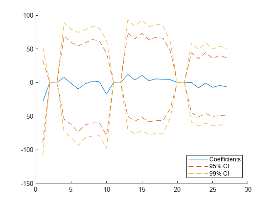
プロットから、係数の 99% 信頼区間の方が 95% 信頼区間よりも幅が広いことがわかります。

入力引数

mdl — 多項回帰モデル オブジェクト

MultinomialRegression モデル オブジェクト

多項回帰モデル オブジェクト。関数 fitmnr で作成される MultinomialRegression モデル オブジェクトとして指定します。

alpha — 有意水準

0.05 (既定値) | 範囲 [0,1] の数値

信頼区間の有意水準。範囲 [0,1] の数値を指定します。ci の信頼水準は 100(1 – alpha)% に等しくなります。alpha は、真の値が信頼区間に含まれない確率です。

例: 0.01

データ型: single | double

出力引数

ci — 信頼区間

数値行列

信頼区間。p 行 2 列の数値行列として返されます。p は係数の個数です。ci の j 番目の行は、mdl の j 番目の係数の信頼区間です。係数 j の名前は、mdl の CoefficientNames プロパティに格納されます。

詳細

信頼区間

係数の信頼区間により回帰係数の推定の精度を測定できます。

100(1 – α)% 信頼区間は、対応する回帰係数が 100(1 – α)% の信頼度になる範囲を与えます。つまり、実験を繰り返すことによって生成される区間の 100(1 – α)% に真の係数値が含まれます。

ソフトウェアは、Wald 法を使用して信頼区間を求めます。回帰係数の 100(1 – α)% 信頼区間は、次のとおりです。

$$b_i\pm t_{\left(1-\alpha /2,n-p\right)}SE\left(b_i\right),$$

ここで、b_i は係数の推定値、SE(b_i) は係数の推定値の標準誤差、t_{(1–α/2,n–p)} は自由度が n – p の t 分布の 100(1 – α/2) 百分位数です。n は観測値の個数、p は回帰係数の個数です。

バージョン履歴

R2023a で導入

参考

MultinomialRegression | fitmnr