nlmefit と nlmefitsa を使用する混合効果のモデル

この例では、混合効果モデルの当てはめ、予測と残差のプロット、結果の解釈を行います。

標本データを読み込みます。

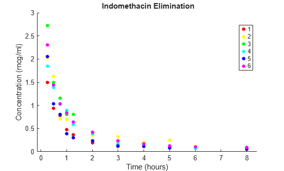
load indomethacin

indomethacin.mat のデータは、被験者 6 人の血流に含まれる薬物インドメタシンの濃度を 8 時間にわたって記録しています。

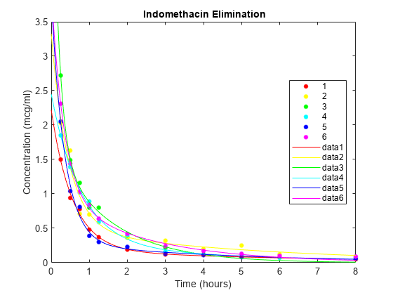
血流中のインドメタシンの散布図を被験者ごとにグループ化してプロットします。

colors = 'rygcbm';
gscatter(time,concentration,subject,colors)
xlabel('Time (hours)')
ylabel('Concentration (mcg/ml)')
title('{\bf Indomethacin Elimination}')
hold on

データが自然なグループになる場合に、モデルに変量効果を含めると効果的です。このデータでは、グループは単に研究対象の個体です。固定効果と変量効果を考慮する混合効果モデルの詳細については、混合効果のモデルを参照してください。

無名関数を使用してモデルを構成します。

model = @(phi,t)(phi(1)*exp(-exp(phi(2))*t) + ...
                 phi(3)*exp(-exp(phi(4))*t));

関数 nlinfit を使用して、被験者に固有の効果を無視し、モデルをすべてのデータに当てはめます。

phi0 = [1 2 1 1];
[phi,res] = nlinfit(time,concentration,model,phi0);

平均二乗誤差を計算します。

numObs = length(time);
numParams = 4;
df = numObs-numParams;
mse = (res'*res)/df

mse = 0.0304

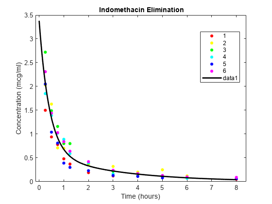
データの散布図にこのモデルを重ね合わせます。

tplot = 0:0.01:8;
plot(tplot,model(phi,tplot),'k','LineWidth',2)
hold off

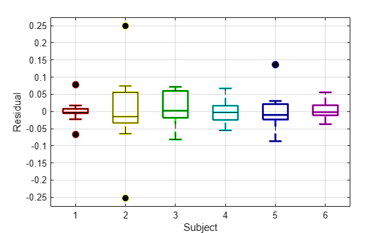
被験者別の残差の箱ひげ図を描画します。

h = boxplot(res,subject,'colors',colors,'symbol','o');
set(h(~isnan(h)),'LineWidth',2)
hold on
boxplot(res,subject,'colors','k','symbol','ko')
grid on
xlabel('Subject')
ylabel('Residual')
hold off

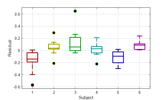
被験者別の残差の箱ひげ図は、ボックスがほとんど 0 の上か下にあることを示し、モデルが被験者に固有の効果を説明できなかったことを示します。

被験者固有の効果を考慮するには、被験者ごとにモデルを個別にデータに当てはめます。

phi0 = [1 2 1 1];
PHI = zeros(4,6);
RES = zeros(11,6);
for I = 1:6
    tI = time(subject == I);
    cI = concentration(subject == I);
    [PHI(:,I),RES(:,I)] = nlinfit(tI,cI,model,phi0);
end
PHI

PHI = 4×6

    2.0293    2.8277    5.4683    2.1981    3.5661    3.0023
    0.5794    0.8013    1.7498    0.2423    1.0408    1.0882
    0.1915    0.4989    1.6757    0.2545    0.2915    0.9685
   -1.7878   -1.6354   -0.4122   -1.6026   -1.5069   -0.8731

平均二乗誤差を計算します。

numParams = 24;
df = numObs-numParams;
mse = (RES(:)'*RES(:))/df

mse = 0.0057

データの散布図をプロットし、被験者別のモデルを重ね合わせます。

gscatter(time,concentration,subject,colors)
xlabel('Time (hours)')
ylabel('Concentration (mcg/ml)')
title('{\bf Indomethacin Elimination}')
hold on
for I = 1:6
    plot(tplot,model(PHI(:,I),tplot),'Color',colors(I))
end
axis([0 8 0 3.5])
hold off

PHI は、6 人の被験者ごとに 4 つのモデル パラメーターの推定を与えます。推定はかなりばらつきますが、データの 24 パラメーター モデルの採用により、平均二乗誤差 0.0057 は、元の 4 パラメーター モデルの 0.0304 よりもかなり減少しています。

被験者別の残差の箱ひげ図を描画します。

h = boxplot(RES,'colors',colors,'symbol','o');
set(h(~isnan(h)),'LineWidth',2)
hold on
boxplot(RES,'colors','k','symbol','ko')
grid on
xlabel('Subject')
ylabel('Residual')
hold off

より大きなモデルによってほとんどの被験者固有の効果が説明できることが箱ひげ図で示されました。残差の広がり (箱ひげ図の垂直のスケール) は前の箱ひげ図よりずっと小さく、ボックスはほぼ 0 に集中するようになります。

24 パラメーター モデルは、研究対象の特定の被験者によって変動を説明できますが、この被験者がより大きい母集団の代表とは見なされません。被験者が描かれる標本分布は、おそらく標本自体より興味深いでしょう。混合効果のモデルの目的は、被験者に固有の変動を母集団の平均付近で変化する変量効果として、より大まかに説明することです。

関数 nlmefit を使用して、混合効果モデルをデータに当てはめます。nlmefit の代わりに nlmefitsa を使用することもできます。

次の無名関数 nlme_model は、異なるパラメーターを個々に使用できるようにすることで、nlinfit が使用する 4 パラメーターのモデルを nlmefit の呼び出し構文に適応させます。既定の設定では、nlmefit は変量効果をすべてのモデル パラメーターに割り当てます。また、既定の設定で、過剰なパラメーター化と関連収束問題を避けるために、nlmefit は対角共分散行列 (変量効果の間の無共分散) を仮定します。

nlme_model = @(PHI,t)(PHI(:,1).*exp(-exp(PHI(:,2)).*t) + ...
                      PHI(:,3).*exp(-exp(PHI(:,4)).*t));
phi0 = [1 2 1 1];
[phi,PSI,stats] = nlmefit(time,concentration,subject, ...
                          [],nlme_model,phi0)

phi = 4×1

    2.8277
    0.7729
    0.4606
   -1.3459

PSI = 4×4

    0.3264         0         0         0
         0    0.0250         0         0
         0         0    0.0124         0
         0         0         0    0.0000

stats = struct with fields:
           dfe: 57
          logl: 54.5882
           mse: 0.0066
          rmse: 0.0787
    errorparam: 0.0815
           aic: -91.1765
           bic: -93.0506
          covb: [4x4 double]
        sebeta: [0.2558 0.1066 0.1092 0.2244]
          ires: [66x1 double]
          pres: [66x1 double]
         iwres: [66x1 double]
         pwres: [66x1 double]
         cwres: [66x1 double]

平均二乗誤差 0.0066 は、変量効果なしの 4 パラメーター モデルの 0.0304 よりかなり良く、変量効果なしの 24 パラメーター モデルの 0.0057 に匹敵します。

推定された共分散行列 PSI は 4 つ目の変量効果の分散が本質的に 0 であることを示し、モデルを単純化するために削除できることを示唆します。これを行うために、名前と値のペア 'REParamsSelect' を使用して、nlmefit 内で変量効果でモデル化するパラメーターのインデックスを指定します。

[phi,PSI,stats] = nlmefit(time,concentration,subject, ...
                          [],nlme_model,phi0, ...
                          'REParamsSelect',[1 2 3])

phi = 4×1

    2.8277
    0.7728
    0.4605
   -1.3460

PSI = 3×3

    0.3270         0         0
         0    0.0250         0
         0         0    0.0124

stats = struct with fields:
           dfe: 58
          logl: 54.5875
           mse: 0.0066
          rmse: 0.0780
    errorparam: 0.0815
           aic: -93.1750
           bic: -94.8410
          covb: [4x4 double]
        sebeta: [0.2560 0.1066 0.1092 0.2244]
          ires: [66x1 double]
          pres: [66x1 double]
         iwres: [66x1 double]
         pwres: [66x1 double]
         cwres: [66x1 double]

対数尤度 logl は、すべてのパラメーターが変量効果のものとほぼ同一です。赤池情報量基準 aic は -91.1765 から -93.1750 に減少します。そして、ベイズ情報量基準 bic は -93.0506 から -94.8410 に減少します。これらの方法は、4 つ目の変量効果を棄却する決定をサポートします。

フルの共分散行列で単純化したモデルの再近似により、変量効果の間で相関関係を識別することができます。これを行うには、CovPattern パラメーターを使用して、共分散行列内で非ゼロの要素のパターンを指定します。

[phi,PSI,stats] = nlmefit(time,concentration,subject, ...
                          [],nlme_model,phi0, ...
                          'REParamsSelect',[1 2 3], ...
                          'CovPattern',ones(3))

phi = 4×1

    2.8149
    0.8292
    0.5613
   -1.1408

PSI = 3×3

    0.4769    0.1152    0.0500
    0.1152    0.0321    0.0032
    0.0500    0.0032    0.0236

stats = struct with fields:
           dfe: 55
          logl: 58.4728
           mse: 0.0061
          rmse: 0.0782
    errorparam: 0.0781
           aic: -94.9457
           bic: -97.2363
          covb: [4x4 double]
        sebeta: [0.3028 0.1104 0.1179 0.1662]
          ires: [66x1 double]
          pres: [66x1 double]
         iwres: [66x1 double]
         pwres: [66x1 double]
         cwres: [66x1 double]

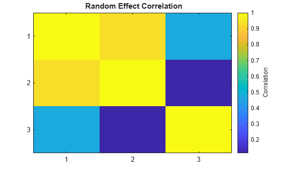
推定された共分散行列 PSI は、最初の 2 つのパラメーターにおける変量効果が比較的強い相関関係をもっていること、そして、両方とも最後の無作為な効果で比較的弱い相関関係をもっていることを示します。corrcov を使用して、PSI を相関関係行列に変換すると、この共分散行列内の構造はより明白になります。

RHO = corrcov(PSI)

RHO = 3×3

    1.0000    0.9316    0.4708
    0.9316    1.0000    0.1180
    0.4708    0.1180    1.0000

clf; 
imagesc(RHO)
set(gca,'XTick',[1 2 3],'YTick',[1 2 3])
title('{\bf Random Effect Correlation}')
h = colorbar;
set(get(h,'YLabel'),'String','Correlation');

共分散パターンの仕様をブロック対角に変更することにより、この構造をモデルに組み入れます。

P = [1 1 0;1 1 0;0 0 1] % Covariance pattern

P = 3×3

     1     1     0
     1     1     0
     0     0     1

[phi,PSI,stats,b] = nlmefit(time,concentration,subject, ...
                            [],nlme_model,phi0, ...
                            'REParamsSelect',[1 2 3], ...
                            'CovPattern',P)

phi = 4×1

    2.7830
    0.8981
    0.6581
   -1.0000

PSI = 3×3

    0.5180    0.1069         0
    0.1069    0.0221         0
         0         0    0.0454

stats = struct with fields:
           dfe: 57
          logl: 58.0804
           mse: 0.0061
          rmse: 0.0768
    errorparam: 0.0782
           aic: -98.1608
           bic: -100.0350
          covb: [4x4 double]
        sebeta: [0.3171 0.1073 0.1384 0.1453]
          ires: [66x1 double]
          pres: [66x1 double]
         iwres: [66x1 double]
         pwres: [66x1 double]
         cwres: [66x1 double]

b = 3×6

   -0.8507   -0.1563    1.0427   -0.7559    0.5652    0.1550
   -0.1756   -0.0323    0.2152   -0.1560    0.1167    0.0320
   -0.2756    0.0519    0.2620    0.1064   -0.2835    0.1389

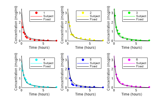
ブロック対角共分散構造は、対数尤度に大きな影響を与えずに、aic を -94.9462 から -98.1608 に減らし、bic を -97.2368 から -100.0350 に減らします。これらの方法は、最終モデル内で使用される共分散構造をサポートします。出力 b は、6 人の被験者ごとに 3 つの変量効果の予測を与えます。これらは phi における固定効果の推定と結合され、混合効果モデルを生成します。

6 人の被験者別に混合効果モデルをプロットします。比較するために、変量効果のないモデルも示されます。

PHI = repmat(phi,1,6) + ...                 % Fixed effects
      [b(1,:);b(2,:);b(3,:);zeros(1,6)];    % Random effects
RES = zeros(11,6); % Residuals
colors = 'rygcbm';
for I = 1:6
    fitted_model = @(t)(PHI(1,I)*exp(-exp(PHI(2,I))*t) + ...
                        PHI(3,I)*exp(-exp(PHI(4,I))*t));
    tI = time(subject == I);
    cI = concentration(subject == I);
    RES(:,I) = cI - fitted_model(tI);
    
    subplot(2,3,I)
    scatter(tI,cI,20,colors(I),'filled')
    hold on
    plot(tplot,fitted_model(tplot),'Color',colors(I))
    plot(tplot,model(phi,tplot),'k')
    axis([0 8 0 3.5])
    xlabel('Time (hours)')
    ylabel('Concentration (mcg/ml)')
    legend(num2str(I),'Subject','Fixed')
end

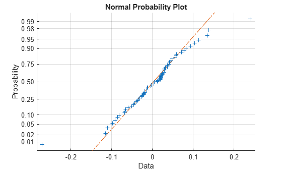
データ内の明らかな外れ値 (前の箱ひげ図を参照) が無視されると、残差の正規確率プロットは、誤差のモデル仮定と妥当な一致を示します。

figure
normplot(RES(:))

参考

nlmefit | nlmefitsa

関連するトピック

• 混合効果のモデル
• モデルの検証のための残差の検査