判別分析分類器の作成と可視化

この例では、フィッシャーのアヤメのデータの線形分類と 2 次分類の実施方法を示します。

標本データを読み込みます。

load fisheriris

列ベクトル species は、3 種類のアヤメ setosa、versicolor、virginica で構成されています。double 行列 meas は、花に関する 4 種類の測定値、がく片の長さと幅 (cm) と花弁の長さと幅 (cm) で構成されています。

花弁の長さ (meas の 3 番目の列) と花弁の幅 (meas の 4 番目の列) の測定値を使用します。これらをそれぞれ変数 PL および変数 PW として保存します。

PL = meas(:,3);
PW = meas(:,4);

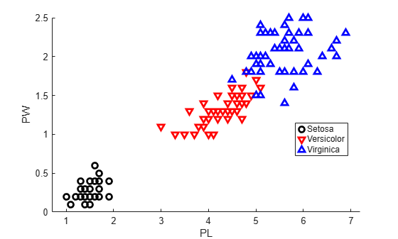
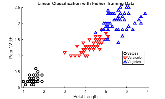
分類を示すデータをプロットします。つまり、種類ごとにグループ化された測定値の散布図を作成します。

h1 = gscatter(PL,PW,species,'krb','ov^',[],'off');
h1(1).LineWidth = 2;
h1(2).LineWidth = 2;
h1(3).LineWidth = 2;
legend('Setosa','Versicolor','Virginica','Location','best')
hold on

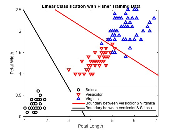
線形分類器を作成します。

X = [PL,PW];
MdlLinear = fitcdiscr(X,species);

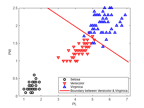
2 番目と 3 番目のクラスの間で線形境界の係数を取得します。

MdlLinear.ClassNames([2 3])

ans = 2x1 cell
    {'versicolor'}
    {'virginica' }

K = MdlLinear.Coeffs(2,3).Const;  
L = MdlLinear.Coeffs(2,3).Linear;

2 番目と 3 番目のクラスを分離する曲線をプロットします。

$$K+\left[\begin{array}{cc}{x}_1& x_2\end{array}\right]L=0.$$

f = @(x1,x2) K + L(1)*x1 + L(2)*x2;
h2 = fimplicit(f,[.9 7.1 0 2.5]);
h2.Color = 'r';
h2.LineWidth = 2;
h2.DisplayName = 'Boundary between Versicolor & Virginica';

1 番目と 2 番目のクラスの間で線形境界の係数を取得します。

MdlLinear.ClassNames([1 2])

ans = 2x1 cell
    {'setosa'    }
    {'versicolor'}

K = MdlLinear.Coeffs(1,2).Const;
L = MdlLinear.Coeffs(1,2).Linear;

1 番目と 2 番目のクラスを分離する曲線をプロットします。

f = @(x1,x2) K + L(1)*x1 + L(2)*x2;
h3 = fimplicit(f,[.9 7.1 0 2.5]);
h3.Color = 'k';
h3.LineWidth = 2;
h3.DisplayName = 'Boundary between Versicolor & Setosa';
axis([.9 7.1 0 2.5])
xlabel('Petal Length')
ylabel('Petal Width')
title('{\bf Linear Classification with Fisher Training Data}')

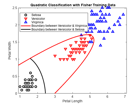
2 次判別分類器を作成します。

MdlQuadratic = fitcdiscr(X,species,'DiscrimType','quadratic');

プロットから線形境界を削除します。

delete(h2);
delete(h3);

2 番目と 3 番目のクラスの間で 2 次境界の係数を取得します。

MdlQuadratic.ClassNames([2 3])

ans = 2x1 cell
    {'versicolor'}
    {'virginica' }

K = MdlQuadratic.Coeffs(2,3).Const;
L = MdlQuadratic.Coeffs(2,3).Linear; 
Q = MdlQuadratic.Coeffs(2,3).Quadratic;

2 番目と 3 番目のクラスを分離する曲線をプロットします。

$$K+\left[\begin{array}{cc}{x}_1& x_2\end{array}\right]L+\left[\begin{array}{cc}{x}_1& x_2\end{array}\right]Q\left[\begin{array}{c}{x}_1\\ x_2\end{array}\right]=0.$$

f = @(x1,x2) K + L(1)*x1 + L(2)*x2 + Q(1,1)*x1.^2 + ...
    (Q(1,2)+Q(2,1))*x1.*x2 + Q(2,2)*x2.^2;
h2 = fimplicit(f,[.9 7.1 0 2.5]);
h2.Color = 'r';
h2.LineWidth = 2;
h2.DisplayName = 'Boundary between Versicolor & Virginica';

1 番目と 2 番目のクラスの間で 2 次境界の係数を取得します。

MdlQuadratic.ClassNames([1 2])

ans = 2x1 cell
    {'setosa'    }
    {'versicolor'}

K = MdlQuadratic.Coeffs(1,2).Const;
L = MdlQuadratic.Coeffs(1,2).Linear; 
Q = MdlQuadratic.Coeffs(1,2).Quadratic;

1 番目と 2 番目のクラスを分離する曲線をプロットします。

f = @(x1,x2) K + L(1)*x1 + L(2)*x2 + Q(1,1)*x1.^2 + ...
    (Q(1,2)+Q(2,1))*x1.*x2 + Q(2,2)*x2.^2;
h3 = fimplicit(f,[.9 7.1 0 1.02]); % Plot the relevant portion of the curve.
h3.Color = 'k';
h3.LineWidth = 2;
h3.DisplayName = 'Boundary between Versicolor & Setosa';
axis([.9 7.1 0 2.5])
xlabel('Petal Length')
ylabel('Petal Width')
title('{\bf Quadratic Classification with Fisher Training Data}')
hold off

参考

関数

• fitcdiscr

オブジェクト

• ClassificationDiscriminant

関連するトピック

• 判別分析による分類