synthesizeTabularData

Synthesize tabular data using binning-based or SMOTE-based synthesizer

Since R2024b

Syntax

syntheticX = synthesizeTabularData(synthesizer,n)

[syntheticX,syntheticY] = synthesizeTabularData(synthesizer,n)

___ = synthesizeTabularData(___,Name=Value)

Description

syntheticX = synthesizeTabularData(synthesizer,n) generates n observations of synthetic data using a trained synthesizer. The function uses the information in synthesizer to return the synthetic data syntheticX.

[syntheticX,syntheticY] = synthesizeTabularData(synthesizer,n) additionally returns the synthetic class labels syntheticY. To return nonempty syntheticY, you must create synthesizer using existing class labels as a separate variable (Y). (since R2026a)

___ = synthesizeTabularData(___,Name=Value) specifies options using one or more name-value arguments in addition to any of the input argument combinations in the previous syntaxes. For example, you can specify the class for which to generate observations and the options for computing in parallel.

Examples

Synthesize Data for Model Training Using binningTabularSynthesizer

Use existing training data to create a binningTabularSynthesizer object. Then, synthesize data using the synthesizeTabularData object function. Train a model using the existing training data, and then train the same type of model using the synthetic data. Compare the performance of the two models using test data.

Load the carbig data set, which contains measurements of cars made in the 1970s and early 1980s. Create a table containing the predictor variables Acceleration, Displacement, and so on, as well as the response variable MPG.

load carbig
tbl = table(Acceleration,Cylinders,Displacement,Horsepower, ...
    Model_Year,Origin,MPG,Weight);

Remove rows of tbl where the table has missing values.

tbl = rmmissing(tbl);

Partition the data into training and test sets. Use approximately 60% of the observations for model training and synthesizing new data, and 40% of the observations for model testing. Use cvpartition to partition the data.

rng("default")
cv = cvpartition(size(tbl,1),"Holdout",0.4);
trainTbl = tbl(training(cv),:);
testTbl = tbl(test(cv),:);

Create a binningTabularSynthesizer object by using the trainTbl data set. The binningTabularSynthesizer function uses binning techniques to learn the distribution of the multivariate data set. Use 20 equal-width bins for each continuous variable. Specify the Cylinders and Model_Year variables as discrete numeric variables.

synthesizer = binningTabularSynthesizer(trainTbl, ...
    BinMethod="equal-width",NumBins=20, ...
    DiscreteNumericVariables=["Cylinders","Model_Year"])

synthesizer = 
  binningTabularSynthesizer

               VariableNames: ["Acceleration"    "Cylinders"    "Displacement"    "Horsepower"    "Model_Year"    "Origin"    "MPG"    "Weight"]
        CategoricalVariables: 6
    DiscreteNumericVariables: [2 5]
             BinnedVariables: [1 3 4 7 8]
                   BinMethod: "equal-width"
                     NumBins: [20 20 20 20 20]
                    BinEdges: {[21×1 double]  [21×1 double]  [21×1 double]  [21×1 double]  [21×1 double]}
             NumObservations: 236


  Properties, Methods

synthesizer is a binningTabularSynthesizer object with five binned variables. Each binned variable has the same number of bins.

Synthesize new data by using synthesizer. Specify to generate 1000 observations.

syntheticTbl = synthesizeTabularData(synthesizer,1000);

The synthesizeTabularData object function uses the data distribution information stored in synthesizer to generate syntheticTbl.

To visualize the difference between the existing data and synthetic data, you can use the detectdrift function. The function uses permutation testing to detect drift between trainTbl and syntheticTbl.

dd = detectdrift(trainTbl,syntheticTbl);

dd is a DriftDiagnostics object with plotEmpiricalCDF and plotHistogram object functions for visualization.

For continuous variables, use the plotEmpiricalCDF function to see the difference between the empirical cumulative distribution function (ecdf) of the values in trainTbl and the ecdf of the values in syntheticTbl.

continuousVariable = "Displacement";
plotEmpiricalCDF(dd,Variable=continuousVariable)
legend(["Real data","Synthetic data"])

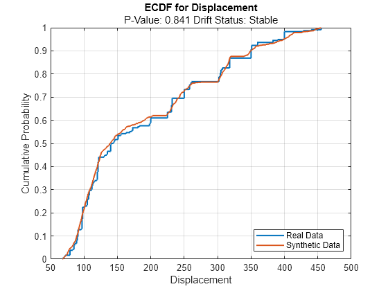
For the Displacement predictor, the ecdf plot for the existing values (in blue) matches the ecdf plot for the synthetic values (in red) fairly well.

For discrete variables, use the plotHistogram function to see the difference between the histogram of the values in trainTbl and the histogram of the values in syntheticTbl.

discreteVariable = "Model_Year";
plotHistogram(dd,Variable=discreteVariable)
legend(["Real data","Synthetic data"])

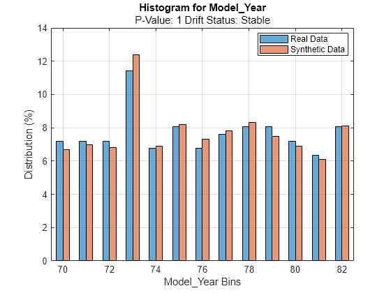
For the Model_Year predictor, the histogram for the existing values (in blue) matches the histogram for the synthetic values (in red) fairly well.

Train a bagged ensemble of trees using the original training data trainTbl. Specify MPG as the response variable. Then, train the same kind of regression model using the synthetic data syntheticTbl.

originalMdl = fitrensemble(trainTbl,"MPG",Method="Bag");
newMdl = fitrensemble(syntheticTbl,"MPG",Method="Bag");

Evaluate the performance of the two models on the test set by computing the test mean squared error (MSE). Smaller MSE values indicate better performance.

originalMSE = loss(originalMdl,testTbl)

originalMSE = 
7.0784

newMSE = loss(newMdl,testTbl)

newMSE = 
6.1031

The model trained on the synthetic data performs slightly better on the test data.

Synthesize Data for Model Training Using smoteTabularSynthesizer

Use existing training data to create a smoteTabularSynthesizer object. Then, synthesize data using the synthesizeTabularData object function. Train a model using the existing training data, and then train the same type of model using both the existing training data and the synthetic data. Compare the performance of the two models using test data.

Load the carbig data set, which contains measurements of cars made in the 1970s and early 1980s. Categorize the cars based on whether they were made in Europe.

load carbig
Origin = categorical(cellstr(Origin));
Origin = mergecats(Origin,["France","Germany", ...
    "Sweden","Italy","England"],"Europe");
Origin = mergecats(Origin,["USA","Japan"],"NotEurope");
tabulate(Origin)

      Value    Count   Percent
     Europe       73     17.98%
  NotEurope      333     82.02%

The data is imbalanced, with only about 18% of cars originating in Europe.

Create a table containing the variables Acceleration, Displacement, and so on, as well as the response variable Origin. Remove rows of cars where the table has missing values.

cars = table(Acceleration,Displacement,Horsepower, ...
    MPG,Weight,Origin);
cars = rmmissing(cars);

Partition the data into training and test sets. Use approximately 50% of the observations for model training and synthesizing new data, and 50% of the observations for model testing. Use stratified partitioning so that approximately the same ratio of European to non-European cars exists in both the training and test sets.

rng("default")
cv = cvpartition(cars.Origin,Holdout=0.5);
trainCars = cars(training(cv),:);
testCars = cars(test(cv),:);

Create a smoteTabularSynthesizer object using the trainCars data set. Specify Origin as the class labels variable.

synthesizer = smoteTabularSynthesizer(trainCars,"Origin")

synthesizer = 
  smoteTabularSynthesizer

      VariableNames: ["Acceleration"    "Displacement"    "Horsepower"    "MPG"    "Weight"]
         ClassNames: [Europe    NotEurope]
       NumNeighbors: [5 5]
           Distance: "seuclidean"
    NumObservations: [34 162]


  Properties, Methods

synthesizer is a smoteTabularSynthesizer object with two classes (Europe and NotEurope).

Synthesize new data by using synthesizer. Specify to generate 40 observations belonging to the class of European cars only.

syntheticCars = synthesizeTabularData(synthesizer,40,ClassNames="Europe");

The synthesizeTabularData object function uses the information stored in synthesizer to generate syntheticCars.

To visualize the difference between the existing European car data and the synthetic European car data, you can use the detectdrift function. Filter the trainCars data to include European car data only. The detectdrift function uses permutation testing to detect drift between europeanCars and syntheticCars.

europeanCars = trainCars(trainCars.Origin=="Europe",:);

dd = detectdrift(europeanCars,syntheticCars);

dd is a DriftDiagnostics object with a plotEmpiricalCDF object function for visualization.

For the continuous variables, use the plotEmpiricalCDF function to see the difference between the empirical cumulative distribution function (ecdf) of the values in europeanCars and the ecdf of the values in syntheticCars.

continuousVariable = "Acceleration";
plotEmpiricalCDF(dd,Variable=continuousVariable)
legend(["Real data","Synthetic data"])

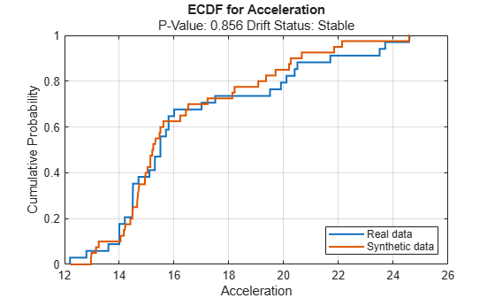
For the Acceleration predictor, the ecdf plot for the existing values (in blue) matches the ecdf plot for the synthetic values (in red) fairly well.

Train an SVM classifier using the original training data trainCars. Specify Origin as the response variable, and standardize the predictors before training. Then, train the same kind of classifier using both the original data and the synthetic data (syntheticCars).

originalMdl = fitcsvm(trainCars,"Origin",Standardize=true);
newMdl = fitcsvm([trainCars;syntheticCars],"Origin",Standardize=true);

Evaluate the performance of the two models on the test set using confusion matrices.

originalPredictions = predict(originalMdl,testCars);
newPredictions = predict(newMdl,testCars);

tiledlayout(1,2)
nexttile
confusionchart(testCars.Origin,originalPredictions)
title("Original Model")
nexttile
confusionchart(testCars.Origin,newPredictions)
title("New Model")

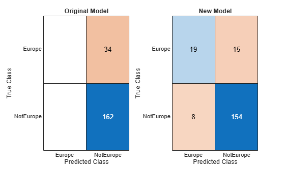
The model trained on the original data classifies all test observations as non-European cars. The model trained on the original and synthetic data has greater accuracy than the other model and correctly classifies the majority of European cars in the test set.

Evaluate Synthetic Data

Evaluate data synthesized from an existing data set. Compare the existing and synthetic data sets to determine the similarity between the two multivariate data distributions.

Load the sample file fisheriris.csv, which contains iris data including sepal length, sepal width, petal width, and species type. Read the file into a table, and then convert the Species variable into a categorical variable. Print a summary of the variables in the table.

fisheriris = readtable("fisheriris.csv");
fisheriris.Species = categorical(fisheriris.Species);
summary(fisheriris)

fisheriris: 150×5 table

Variables:

    SepalLength: double
    SepalWidth: double
    PetalLength: double
    PetalWidth: double
    Species: categorical (3 categories)

Statistics for applicable variables:

                   NumMissing       Min          Median         Max           Mean          Std    

    SepalLength        0           4.3000        5.8000        7.9000        5.8433        0.8281  
    SepalWidth         0                2             3        4.4000        3.0573        0.4359  
    PetalLength        0                1        4.3500        6.9000        3.7580        1.7653  
    PetalWidth         0           0.1000        1.3000        2.5000        1.1993        0.7622  
    Species            0                                                                           

The summary display includes statistics for each variable. For example, the sepal length values range from 4.3 to 7.9, with a median of 5.8.

Create 150 new observations from the data in fisheriris. First, create an object by using the binningTabularSynthesizer function. Then, synthesize the data by using the synthesizeTabularData object function. Print a summary of the variables in the new syntheticData data set.

rng(0,"twister") % For reproducibility
synthesizer = binningTabularSynthesizer(fisheriris);
syntheticData = synthesizeTabularData(synthesizer,150);
summary(syntheticData)

syntheticData: 150×5 table

Variables:

    SepalLength: double
    SepalWidth: double
    PetalLength: double
    PetalWidth: double
    Species: categorical (3 categories)

Statistics for applicable variables:

                   NumMissing       Min          Median         Max           Mean          Std    

    SepalLength        0           4.3079        5.7174        7.6399        5.8280        0.8576  
    SepalWidth         0           2.0236        3.0336        4.2866        3.0819        0.4572  
    PetalLength        0           1.0010        4.4453        6.8538        3.6572        1.8192  
    PetalWidth         0           0.1002        1.3502        2.4759        1.1719        0.7597  
    Species            0                                                                           

You can compare the variable statistics for syntheticData to the variable statistics for fisheriris. For example, the sepal length values in the synthetic data set range from approximately 4.3 to 7.6, with a median of 5.7. These statistics are similar to the statistics in the fisheriris data set.

Visually compare the observations in fisheriris and syntheticData by using scatter plots. Each point corresponds to an observation. The point color indicates the species of the corresponding iris.

tiledlayout(1,2)
nexttile
gscatter(fisheriris.SepalLength,fisheriris.PetalLength,fisheriris.Species)
xlabel("Sepal Length")
ylabel("Petal Length")
title("Existing Data")
nexttile
gscatter(syntheticData.SepalLength,syntheticData.PetalLength,syntheticData.Species)
xlabel("Sepal Length")
ylabel("Petal Length")
title("Synthetic Data")

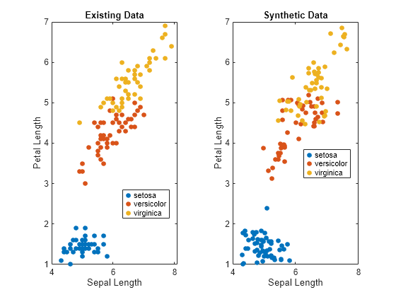
The scatter plots indicate that the existing data set and the synthetic data set have similar characteristics.

Compare the existing and synthetic data sets by using the mmdtest function. The function performs a two-sample hypothesis test for the null hypothesis that the data sets come from the same distribution.

[mmd2,p,h] = mmdtest(fisheriris,syntheticData)

mmd2 = 
0.0020

p = 
0.9600

h = 
0

The returned value of h = 0 indicates that mmdtest fails to reject the null hypothesis that the data sets come from different distributions at the significance level of 5%. As with other hypothesis tests, this result does not guarantee that the null hypothesis is true. That is, the data sets do not necessarily come from the same distribution, but the low mmd2 value (square maximum mean discrepancy) and the high p-value indicate that the distributions of the real and synthetic data sets are similar.

Input Arguments

synthesizer — Trained synthesizer

binningTabularSynthesizer object | smoteTabularSynthesizer object

Trained synthesizer, specified as a binningTabularSynthesizer or smoteTabularSynthesizer object.

n — Number of synthetic data observations to generate

positive integer scalar | two-element positive integer vector

Number of synthetic data observations to generate, specified as a positive integer scalar or a two-element positive integer vector.

To generate synthetic data for two classes, you can specify n as a two-element vector. Each element indicates the number of observations to generate for the corresponding class in ClassNames. If you specify n as a scalar, then the software generates synthetic observations for the two classes with approximately the same proportion found in synthesizer.NumObservations. (since R2026a)

Example: 100

Data Types: single | double

Name-Value Arguments

Specify optional pairs of arguments as Name1=Value1,...,NameN=ValueN, where Name is the argument name and Value is the corresponding value. Name-value arguments must appear after other arguments, but the order of the pairs does not matter.

Example: synthesizeTabularData(synthesizer,10,ClassNames="b",Options=statset(UseParallel=true)) specifies to generate 10 synthetic observations for class "b" in parallel.

ClassNames — Names of classes

numeric vector | categorical vector | logical vector | character array | string array | cell array of character vectors | []

Since R2026a

Names of the classes for which to generate synthetic data, specified as a numeric, categorical, or logical vector; a character or string array; or a cell array of character vectors.

You can use ClassNames to:

• Specify the order of the classes.

• Select a class for generating synthetic data. For example, suppose that the set of distinct class labels is ["b","g"]. To generate synthetic observations from class "g" only, specify ClassNames="g".

The default value for ClassNames is the ordered set of distinct class labels in the class labels variable used to create synthesizer.

Example: ClassNames=["g","b"]

Data Types: single | double | logical | char | string | cell | categorical

Options — Options for computing in parallel and setting random streams

structure

Options for computing in parallel and setting random streams, specified as a structure. Create the Options structure using statset. This table lists the option fields and their values.

Field Name	Value	Default
UseParallel	Set this value to true to run computations in parallel.	false
UseSubstreams	Set this value to true to run computations in a reproducible manner. To compute reproducibly, set Streams to a type that allows substreams: "mlfg6331_64" or "mrg32k3a".	false
Streams	Specify this value as a RandStream object or cell array of such objects. Use a single object except when the UseParallel value is true and the UseSubstreams value is false. In that case, use a cell array that has the same size as the parallel pool.	If you do not specify Streams, then synthesizeTabularData uses the default stream or streams.

Note

You need Parallel Computing Toolbox™ to run computations in parallel.

Example: Options=statset(UseParallel=true,UseSubstreams=true,Streams=RandStream("mlfg6331_64"))

Data Types: struct

Output Arguments

syntheticX — Synthetic data set

numeric matrix | table

Synthetic data set, returned as a numeric matrix or a table. syntheticX has the same data type as the data used to create synthesizer.

If you used Yname to create synthesizer, then the last column of the syntheticX table contains the class labels for the synthetic data set. (since R2026a)

syntheticY — Synthetic class labels

numeric vector | categorical vector | logical vector | character array | string array | cell array of character vectors

Since R2026a

Synthetic class labels, returned as a numeric, categorical, or logical vector; a character or string array; or a cell array of character vectors. syntheticY has the same data type as the class labels used to create synthesizer.

Algorithms

Generate Synthetic Data Using Binning

When you use a binning technique, the process for estimating the multivariate data distribution includes computing the probability of each unique row in the one-hot encoded data set (after binning continuous variables). The synthesizeTabularData function uses this estimated multivariate data distribution to generate synthetic observations. The function performs these steps:

1. Use the previously computed probabilities to sample with replacement n rows from the unique rows in the encoded data set.

2. Decode the sampled data to obtain the bin indices (for continuous variables) and categories (for discrete variables).

3. For the binned variables, uniformly sample from within the bin edges to obtain continuous values. If you use equiprobable binning (BinMethod) and the extreme bin widths are greater than 1.5 times the median of the nonextreme bin widths, then the function samples from the cumulative distribution function (cdf) in the extreme bins.

Generate Synthetic Data Using SMOTE

SMOTE (synthetic minority oversampling technique) is a technique for generating synthetic data when you have an imbalanced data set, that is, when the number of observations is not uniform across the response classes.

Assume the data set X has two classes, where class k_big has many more observations than class k_small. If the data set X has only one class, then assume all observations belong to k_small. When you use SMOTE, the synthesizeTabularData function generates each new k_small observation in the following way:

1. Randomly select an observation x in k_small.

2. In the data set, find the NumNeighbors-nearest neighbors of x that also belong to k_small.

3. Randomly select one of the nearest neighbors $$\widehat{x}$$.

4. For each continuous predictor p, set the predictor value of the new observation to $$x_p+r({\widehat{x}}_p-x_p)$$, where x_p is the predictor value of the original observation x, $${\widehat{x}}_p$$ is the predictor value of the nearest neighbor $$\widehat{x}$$, and r is a random value in (0,1) as selected by the rand function.

   For the categorical predictors q₁, …, q_m, set the predictor values of the new observation to the mode of the vector of predictor values among the NumNeighbors-nearest neighbors of x. In the case of a tie, choose a vector at random.

The function follows the same process to generate observations in class k_big. The number of synthetic observations generated depends on n (the input argument of synthesizeTabularData).

References

[1] Chawla, Nitesh V., Kevin W. Bowyer, Lawrence O. Hall, and W. Philip Kegelmeyer. "SMOTE: Synthetic Minority Over-sampling Technique." Journal of Artificial Intelligence Research 16 (2002): 321-357.

Extended Capabilities

Automatic Parallel Support

Accelerate code by automatically running computation in parallel using Parallel Computing Toolbox™.

To run in parallel, specify the Options name-value argument in the call to this function and set the UseParallel field of the options structure to true using statset:

Options=statset(UseParallel=true)

For more information about parallel computing, see Run MATLAB Functions with Automatic Parallel Support (Parallel Computing Toolbox).

Version History

Introduced in R2024b

R2026a: Generate synthetic data for imbalanced data sets using SMOTE

You can use the synthetic minority oversampling technique (SMOTE) algorithm to generate synthetic data for binary classification. Using SMOTE can be helpful when you have imbalanced data, that is, when one class contains many more observations than the other.

First, create a smoteTabularSynthesizer object. You can adjust parameters of the SMOTE technique by using the NumNeighbors, Distance, and CacheSize name-value arguments. Then call the synthesizeTabularData object function to synthesize data using the object.

Regardless of whether you use a binningTabularSynthesizer or smoteTabularSynthesizer object, the synthesizeTabularData function can return synthetic observations for one or two classes. Use the Yname or Y input argument when you create the object, and the ClassNames name-value argument when you call synthesizeTabularData.