このページは機械翻訳を使用して翻訳されました。最新版の英語を参照するには、ここをクリックします。

衛星コンスタレーションのカバー範囲マップ

この例では、衛星シナリオと 2D マップを使用して、関心領域の範囲マップを表示する方法を示します。衛星の カバレッジ マップ には、エリア内の地上受信機へのダウンリンクのエリア全体の受信電力が含まれます。

Mapping Toolbox ™ のマッピング機能と Satellite Communications Toolbox の衛星シナリオ機能を組み合わせることで、等高線付きのカバレッジ マップを作成し、等高線データを可視化および解析に使用できます。この例では、以下を行う方法を説明します。

• 地上局受信機のグリッドを含む衛星シナリオを使用して、カバレッジ マップ データを計算します。

• axesm- ベースのマップやマップ軸などのさまざまなマップ表示を使用してカバレッジ マップを表示します。

• 関心のある他の時間帯のカバレッジ マップを計算して表示します。

シナリオの作成と可視化

衛星シナリオとビューアーを作成します。シナリオの開始日と 1 時間の期間を指定します。

startTime = datetime(2023,2,21,18,0,0);
stopTime = startTime + hours(1);
sampleTime = 60; % seconds
sc = satelliteScenario(startTime,stopTime,sampleTime);
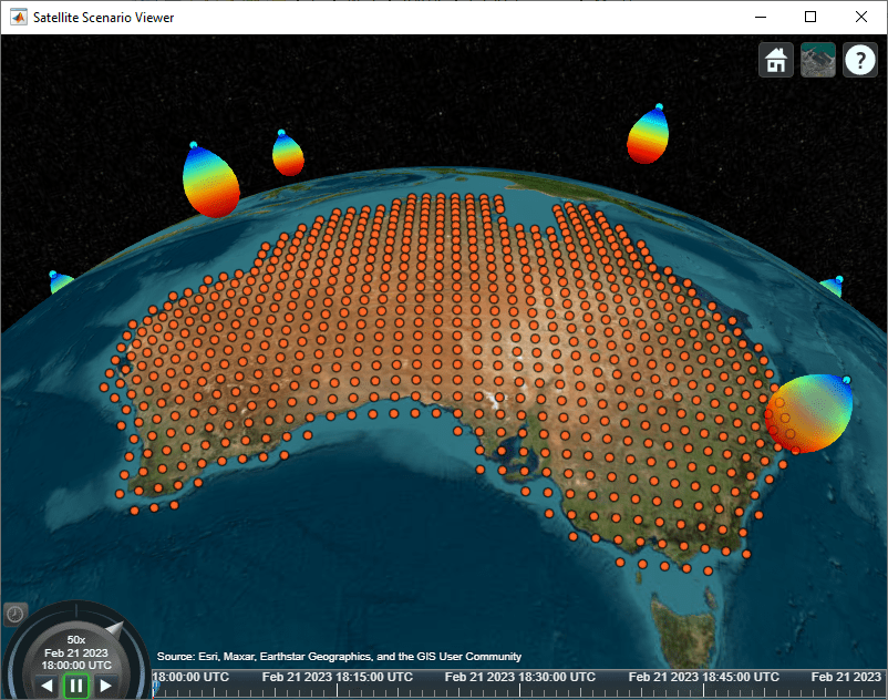
viewer = satelliteScenarioViewer(sc,ShowDetails=false);

衛星コンスタレーションの追加

2018年から2019年にかけて打ち上げられたイリジウムNEXT衛星ネットワーク[1]には、以下の66機の稼働中のLEO衛星が含まれています。

• 約86.6度の傾斜角を持つ6つの軌道面があり、面間のRAANの差は約30度です[1]。

• 軌道面あたり11個の衛星があり、衛星間の真近点角の差はおおよそ32.7度です[1]。

アクティブな Iridium NEXT衛星をシナリオに追加します。イリジウム ネットワーク内の衛星の軌道要素を作成し、衛星を作成します。

numSatellitesPerOrbitalPlane = 11;
numOrbits = 6;

orbitIdx = repelem(1:numOrbits,1,numSatellitesPerOrbitalPlane);
planeIdx = repmat(1:numSatellitesPerOrbitalPlane,1,numOrbits);

RAAN = 180*(orbitIdx-1)/numOrbits;
trueanomaly = 360*(planeIdx-1 + 0.5*(mod(orbitIdx,2)-1))/numSatellitesPerOrbitalPlane;
semimajoraxis = repmat((6371 + 780)*1e3,size(RAAN)); % meters
inclination = repmat(86.4,size(RAAN)); % degrees
eccentricity = zeros(size(RAAN)); % degrees
argofperiapsis = zeros(size(RAAN)); % degrees

iridiumSatellites = satellite(sc,...
    semimajoraxis,eccentricity,inclination,RAAN,argofperiapsis,trueanomaly,...
    Name="Iridium " + string(1:66)');

Aerospace Toolbox ™ のライセンスをお持ちの場合は、walkerStar (Aerospace Toolbox) 関数を使用して Iridiumコンスタレーションを作成することもできます。

オーストラリア周辺の関心領域を定義する

オーストラリアを囲む関心領域 (AOI) を作成して、カバレッジ マップを計算する準備をします。

世界の陸地面積を含むシェイプファイルを地理空間テーブルとしてワークスペースに読み込みます。地理空間テーブルは、地理座標のポリゴン形状を使用して土地面積を表します。オーストラリアのポリゴン形状を抽出します。

landareas = readgeotable("landareas.shp");
australia = geocode("Australia",landareas);

オーストラリアの陸地の周囲に 1 度のバッファ領域を含む地理座標で新しいポリゴン シェイプを作成します。バッファにより、カバレッジ マップの範囲が陸地領域をカバーできるようになります。

bufwidth = 1; % degrees
aoi = buffer(australia.Shape,bufwidth);

AOIをカバーする地上局のグリッドを追加する

AOI をカバーする地上局受信機のグリッドの信号強度を計算して、カバレッジ マップ データを作成します。緯度経度座標のグリッドを作成し、AOI 内の座標を選択して地上局の場所を作成します。

AOI の緯度と経度の制限を計算し、度単位で間隔を指定します。この間隔によって地上局間の距離が決まります。間隔の値が小さいほど、カバレッジ マップの解像度は向上しますが、計算時間も長くなります。

[latlim, lonlim] = bounds(aoi);
spacingInLatLon = 1; % degrees

オーストラリアに適した投影座標参照系 (CRS) を作成します。投影された CRS は、物理的な場所に直交座標 x および y マップ座標を割り当てる情報を提供します。ランベルト正角円錐図法を使用するオーストラリアに適した GDA2020 / GA LCC 投影 CRS を使用します。

proj = projcrs(7845);

データ グリッドの投影された X-Y マップ座標を計算します。グリッド位置間の距離の変動を減らすには、緯度経度座標の代わりに投影された X-Y マップ座標を使用します。

spacingInXY = deg2km(spacingInLatLon)*1000; % meters
[xlimits,ylimits] = projfwd(proj,latlim,lonlim);
R = maprefpostings(xlimits,ylimits,spacingInXY,spacingInXY);
[X,Y] = worldGrid(R);

グリッドの位置を緯度経度座標に変換します。

[gridlat,gridlon] = projinv(proj,X,Y);

AOI 内のグリッド座標を選択します。

gridpts = geopointshape(gridlat,gridlon);
inregion = isinterior(aoi,gridpts);

gslat = gridlat(inregion);
gslon = gridlon(inregion);

座標の地上局を作成します。

gs = groundStation(sc,gslat,gslon);

送信機と受信機を追加する

衛星に送信機を追加し、地上局に受信機を追加することで、ダウンリンクのモデリングを有効にします。

イリジウムコンスタレーションは48ビームのアンテナを使用します。ガウス アンテナまたはカスタム 48ビームアンテナ (Phased Array System Toolbox ™ が必要) を選択します。ガウスアンテナは、イリジウム半視野角62.7度を使用して48ビームアンテナを近似します[1]。アンテナを天底方向に向けます。

fq = 1625e6; % Hz
txpower = 20; % dBW
antennaType = "Gaussian";
halfBeamWidth = 62.7; % degrees

ガウスアンテナを備えた衛星送信機を追加します。

if antennaType == "Gaussian"
    lambda = physconst('lightspeed')/fq; % meters
    dishD = (70*lambda)/(2*halfBeamWidth); % meters
    tx = transmitter(iridiumSatellites, ...
        Frequency=fq, ...
        Power=txpower); 
    gaussianAntenna(tx,DishDiameter=dishD);
end

カスタム 48ビームアンテナを備えた衛星送信機を追加します。ヘルパー関数 helperCustom48BeamAntenna は、サポート ファイルとして例に含まれています。

if antennaType == "Custom 48-Beam"
    antenna = helperCustom48BeamAntenna(fq);
    tx = transmitter(iridiumSatellites, ...
        Frequency=fq, ...
        MountingAngles=[0,-90,0], ... % [yaw, pitch, roll] with -90 using Phased Array System Toolbox convention
        Power=txpower, ...
        Antenna=antenna);  
end

地上局受信機を追加する

等方性アンテナを備えた地上局受信機を追加します。

isotropic = arrayConfig(Size=[1 1]);
rx = receiver(gs,Antenna=isotropic);

衛星送信機のアンテナパターンを可視化します。この可視化では、アンテナが天底を向いている方向が示されています。

pattern(tx,Size=500000);

ラスターカバレッジマップデータの計算

衛星シナリオビューアを閉じて、シナリオの開始時間に対応するカバレッジデータを計算します。satcoverage ヘルパー関数は、グリッド化されたカバレッジ データを返します。この関数は、各衛星について視野の形状を計算し、衛星視野内の各地上局受信機の信号強度を計算します。カバレッジ データは、任意の衛星から受信した最大信号強度です。

delete(viewer)
maxsigstrength = satcoverage(gridpts,sc,startTime,inregion,halfBeamWidth);

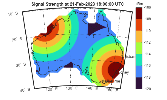
axesm ベースのマップでカバレッジを可視化する

オーストラリアに対応する axesm ベースのマップ上にラスター カバレッジ マップ データをプロットします。マップ軸はベクター データのみのプロットをサポートするのに対し、axesm ベースのマップはベクター データとラスター データの混合のプロットをサポートするため、使用されます。

ディスプレイの最小および最大電力レベルを定義します。

minpowerlevel = -120; % dBm
maxpowerlevel = -106; % dBm

オーストラリアの世界地図を作成し、ラスター カバレッジ マップ データをコンター表示としてプロットします。

figure
worldmap(latlim,lonlim)
mlabel south

colormap turbo
clim([minpowerlevel maxpowerlevel])
geoshow(gridlat,gridlon,maxsigstrength,DisplayType="contour",Fill="on")
geoshow(australia,FaceColor="none")

cBar = contourcbar;
title(cBar,"dBm");
title("Signal Strength at " + string(startTime) + " UTC")

シドニー、メルボルン、ブリスベンの各都市のテキスト ラベルを追加します。geocode 関数を使用して各都市の座標を取得します。

sydneyT = geocode("Sydney,Australia","city");
sydney = sydneyT.Shape;
melbourneT = geocode("Melbourne,Australia","city");
melbourne = melbourneT.Shape;
brisbaneT = geocode("Brisbane,Australia","city");
brisbane = brisbaneT.Shape;

textm(sydney.Latitude,sydney.Longitude,"Sydney")
textm(melbourne.Latitude,melbourne.Longitude,"Melbourne")
textm(brisbane.Latitude,brisbane.Longitude,"Brisbane")

カバレッジマップのコンターを計算する

ラスター カバレッジ マップ データをコンター、カバレッジ マップコンターの地理空間テーブルを作成します。各カバレッジ マップ コンターは、地理座標のポリゴン形状を含む地理空間テーブルの行として表されます。カバレッジ マップの等高線は、可視化と解析の両方に使用できます。

levels = linspace(minpowerlevel,maxpowerlevel,8);
GT = contourDataGrid(gridlat,gridlon,maxsigstrength,levels,proj);
GT = sortrows(GT,"Power (dBm)");
disp(GT)

       Shape        Area (sq km)    Power (dBm)    Power Range (dBm)
    ____________    ____________    ___________    _________________

    geopolyshape     8.5438e+06        -120          -120    -118   
    geopolyshape     8.2537e+06        -118          -118    -116   
    geopolyshape     5.5607e+06        -116          -116    -114   
    geopolyshape     3.6842e+06        -114          -114    -112   
    geopolyshape     2.2841e+06        -112          -112    -110   
    geopolyshape     1.1843e+06        -110          -110    -108   
    geopolyshape     3.8307e+05        -108          -108    -106   

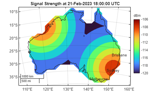
マップ軸上でカバレッジを可視化する

オーストラリアに対応する地図投影を使用して、カバレッジ マップのコンターを地図軸上にプロットします。詳細については、Choose a 2-D Map Display (Mapping Toolbox)を参照してください。

figure
newmap(proj)
hold on

colormap turbo
clim([minpowerlevel maxpowerlevel])
geoplot(GT,ColorVariable="Power (dBm)",EdgeColor="none")
geoplot(australia,FaceColor="none")

cBar = colorbar;
title(cBar,"dBm");
title("Signal Strength at " + string(startTime) + " UTC")

text(sydney.Latitude,sydney.Longitude,"Sydney",HorizontalAlignment="center")
text(melbourne.Latitude,melbourne.Longitude,"Melbourne",HorizontalAlignment="center")
text(brisbane.Latitude,brisbane.Longitude,"Brisbane",HorizontalAlignment="center")

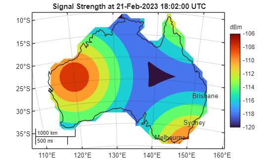
異なる関心時間の範囲を計算して可視化する

異なる関心時間を指定して、カバレッジを計算して可視化します。

secondTOI = startTime + minutes(2); % 2 minutes after the start of the scenario
maxsigstrength = satcoverage(gridpts,sc,secondTOI,inregion,halfBeamWidth);

GT2 = contourDataGrid(gridlat,gridlon,maxsigstrength,levels,proj);
GT2 = sortrows(GT2,"Power (dBm)");

figure
newmap(proj)
hold on

colormap turbo
clim([minpowerlevel maxpowerlevel])
geoplot(GT2,ColorVariable="Power (dBm)",EdgeColor="none")
geoplot(australia,FaceColor="none")

cBar = colorbar;
title(cBar,"dBm");
title("Signal Strength at " + string(secondTOI) + " UTC")

text(sydney.Latitude,sydney.Longitude,"Sydney",HorizontalAlignment="center")
text(melbourne.Latitude,melbourne.Longitude,"Melbourne",HorizontalAlignment="center")
text(brisbane.Latitude,brisbane.Longitude,"Brisbane",HorizontalAlignment="center")

都市のカバー率を計算する

オーストラリアの 3 つの都市のカバレッジ レベルを計算して表示します。

covlevels1 = [coveragelevel(sydney,GT); coveragelevel(melbourne,GT); coveragelevel(brisbane,GT)];
covlevels2 = [coveragelevel(sydney,GT2); coveragelevel(melbourne,GT2); coveragelevel(brisbane,GT2)];

covlevels = table(covlevels1,covlevels2, ...
    RowNames=["Sydney" "Melbourne" "Brisbane"], ...
    VariableNames=["Signal Strength at T1 (dBm)" "Signal Strength T2 (dBm)"])

covlevels=3×2 table
                 Signal Strength at T1 (dBm)    Signal Strength T2 (dBm)
                 ___________________________    ________________________

    Sydney                  -108                          -112          
    Melbourne               -112                          -110          
    Brisbane                -112                          -116          

補助関数

satcoverage ヘルパー関数はカバレッジ データを返します。この関数は、各衛星について視野の形状を計算し、衛星視野内の各地上局受信機の信号強度を計算します。カバレッジ データは、任意の衛星から受信した最大信号強度です。

function coveragedata = satcoverage(gridpts,sc,timeIn,inregion,halfBeamWidth)

    % Get satellites and ground station receivers
    sats = sc.Satellites;
    rxs = [sc.GroundStations.Receivers];

    % Get field-of-view shapes for all satellites
    fovs = satfov(sats,timeIn,halfBeamWidth);

    % Initialize coverage data
    coveragedata = NaN(size(gridpts));

    for satind = 1:numel(sats)
        fov = fovs(satind);

        % Find grid and rx locations which are within the satellite field-of-view
        gridInFOV = isinterior(fov,gridpts);
        rxInFOV = gridInFOV(inregion);

        % Compute sigstrength at grid locations using temporary link objects
        gridsigstrength = NaN(size(gridpts));
        if any(rxInFOV)
            tx = sats(satind).Transmitters;
            lnks = link(tx,rxs(rxInFOV));
            rxsigstrength = sigstrength(lnks,timeIn)+30; % Convert from dBW to dBm
            gridsigstrength(inregion & gridInFOV) = rxsigstrength;
            delete(lnks)
        end

        % Update coverage data with maximum signal strength found
        coveragedata = max(gridsigstrength,coveragedata);
    end
end

satfov ヘルパー関数は、天底指向と球状地球モデルを想定して、各衛星の視野を表す geopolyshape オブジェクトの配列を返します。

function fovs = satfov(sats,timeIn,halfViewAngle)

    % Compute the latitude, longitude, and altitude of all satellites at the input time
    satstates = states(sats,timeIn,CoordinateFrame="geographic");

    fovs = createArray([1 numel(sats)],"geopolyshape");
    for satind = 1:numel(sats)
        lla = satstates(:,1,satind);

        % Find the Earth central angle using the beam view angle
        if isreal(acosd(sind(halfViewAngle)*(lla(3)+earthRadius)/earthRadius))
            % Case when Earth FOV is bigger than antenna FOV
            earthCentralAngle = 90-acosd(sind(halfViewAngle)*(lla(3)+earthRadius)/earthRadius)-halfViewAngle;
        else
            % Case when antenna FOV is bigger than Earth FOV
            earthCentralAngle = 90-halfViewAngle;
        end

        % Create a circular geopolyshape centered at the position of the satellite 
        % with a buffer of width equaling the Earth central angle
        fovs(satind) = aoicircle(lla(1),lla(2),earthCentralAngle);
    end
end

contourDataGrid ヘルパー関数はデータ グリッドのコンター、結果を地理空間テーブルとして返します。表の各行は電力レベルに対応しており、コンターの形状、コンターの形状の面積（平方キロメートル）、レベルの最小電力、およびレベルの電力範囲が含まれます。

function GT = contourDataGrid(latd,lond,data,levels,proj)

    % Pad each side of the grid to ensure no contours extend past the grid bounds
    lond = [2*lond(1,:)-lond(2,:); lond; 2*lond(end,:)-lond(end-1,:)];
    lond = [2*lond(:,1)-lond(:,2) lond 2*lond(:,end)-lond(:,end-1)];
    latd = [2*latd(1,:)-latd(2,:); latd; 2*latd(end,:)-latd(end-1,:)];
    latd = [2*latd(:,1)-latd(:,2) latd 2*latd(:,end)-latd(:,end-1)];
    data = [ones(size(data,1)+2,1)*NaN [ones(1,size(data,2))*NaN; data; ones(1,size(data,2))*NaN] ones(size(data,1)+2,1)*NaN];
    
    % Replace NaN values in power grid with a large negative number
    data(isnan(data)) = min(levels) - 1000;
    
    % Project the coordinates using an equal-area projection
    [xd,yd] = projfwd(proj,latd,lond);
    
    % Contour the projected data
    fig = figure("Visible","off");
    obj = onCleanup(@()close(fig));
    c = contourf(xd,yd,data,LevelList=levels);
    
    % Initialize variables
    x = c(1,:);
    y = c(2,:);
    n = length(y);
    k = 1;
    index = 1;
    levels = zeros(n,1);
    latc = cell(n,1);
    lonc = cell(n,1);
    
    % Process the coordinates of the projected contours
    while k < n
        level = x(k);
        numVertices = y(k);
        yk = y(k+1:k+numVertices);
        xk = x(k+1:k+numVertices);
        k = k + numVertices + 1;
    
        [first,last] = findNanDelimitedParts(xk);
        jindex = 0;
        jy = {};
        jx = {};
    
        for j = 1:numel(first)
            % Process the j-th part of the k-th level
            s = first(j);
            e = last(j);
            cx = xk(s:e);
            cy = yk(s:e);
            if cx(end) ~= cx(1) && cy(end) ~= cy(1)
                cy(end+1) = cy(1); %#ok<*AGROW>
                cx(end+1) = cx(1);
            end
    
            if j == 1 && ~ispolycw(cx,cy)
                % First region must always be clockwise
                [cx,cy] = poly2cw(cx,cy);
            end
    
            % Filter regions made of collinear points or fewer than 3 points
            if ~(length(cx) < 4 || all(diff(cx) == 0) || all(diff(cy) == 0))
                jindex = jindex + 1;
                jy{jindex,1} = cy(:)';
                jx{jindex,1} = cx(:)';
            end
        end
    
        % Unproject the coordinates of the processed contours
        [jx,jy] = polyjoin(jx,jy);
        if length(jy) > 2 && length(jx) > 2
            [jlat,jlon] = projinv(proj,jx,jy);
            latc{index,1} = jlat(:)';
            lonc{index,1} = jlon(:)';
            levels(index,1) = level;
            index = index + 1;
        end
    end
    
    % Create contour shapes from the unprojected coordinates. Include the
    % contour shapes, the areas of the shapes, and the power levels in a
    % geospatial table.
    latc = latc(1:index-1);
    lonc = lonc(1:index-1);
    Shape = geopolyshape(latc,lonc);
    
    Area = area(Shape);
    
    levels = levels(1:index-1);
    Levels = levels;
    
    allPartsGT = table(Shape,Area,Levels);
    
    % Condense the geospatial table into a new geospatial table with one
    % row per power level.
    GT = table.empty;
    levels = unique(allPartsGT.Levels);
    for k = 1:length(levels)
        gtLevel = allPartsGT(allPartsGT.Levels == levels(k),:);
        tLevel = geotable2table(gtLevel,["Latitude","Longitude"]);
        [lon,lat] = polyjoin(tLevel.Longitude,tLevel.Latitude);
        Shape = geopolyshape(lat,lon);
        Levels = levels(k);
        Area = area(Shape);
        GT(end+1,:) = table(Shape,Area,Levels);
    end
    
    maxLevelDiff = max(abs(diff(GT.Levels)));
    LevelRange = [GT.Levels GT.Levels + maxLevelDiff];
    GT.LevelRange = LevelRange;
    
    % Clean up the geospatial table
    GT.Area = GT.Area/1e6;
    GT.Properties.VariableNames = ...
        ["Shape","Area (sq km)","Power (dBm)","Power Range (dBm)"];
end

coveragelevel 関数は、geopointshape オブジェクトのカバレッジ レベルを返します。

function powerLevels = coveragelevel(point,GT)

    % Determine whether points are within coverage
    inContour = false(length(GT.Shape),1);
    for k = 1:length(GT.Shape)
        inContour(k) = isinterior(GT.Shape(k),point);
    end

    % Find the highest coverage level containing the point
    powerLevels = max(GT.("Power (dBm)")(inContour));

    % Return -inf if the point is not contained within any coverage level
    if isempty(powerLevels)
        powerLevels = -inf;
    end
end

findNanDelimitedParts ヘルパー関数は、配列 x の NaN で区切られた各部分の最初の要素と最後の要素のインデックスを見つけます。

function [first,last] = findNanDelimitedParts(x)

    % Find indices of the first and last elements of each part in x. 
    % x can contain runs of multiple NaNs, and x can start or end with 
    % one or more NaNs.

    n = isnan(x(:));
    
    firstOrPrecededByNaN = [true; n(1:end-1)];
    first = find(~n & firstOrPrecededByNaN);
    
    lastOrFollowedByNaN = [n(2:end); true];
    last = find(~n & lastOrFollowedByNaN);
end

参照

[1] Attachment EngineeringStatement SAT-MOD-20131227-00148. https://fcc.report/IBFS/SAT-MOD-20131227-00148/1031348. Accessed 17 Jan. 2023.

参考

aoicircle (Mapping Toolbox)

トピック

• Read Quantitative Data from WMS Server (Mapping Toolbox)