txlineMicrostrip
Create microstrip transmission line
Description
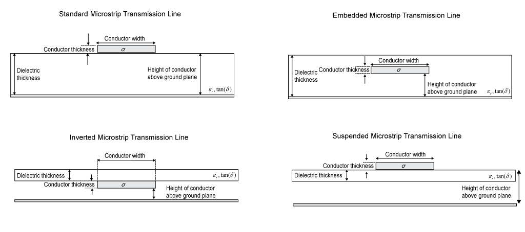
Use the txlineMicrostrip object to create a standard, embedded,
inverted, or suspended microstrip transmission line. This figure shows the cross sections of
the four types of microstrip transmission lines you can create using the
txlineMircostrip object. The physical characteristics of the microstrip
transmission line include the conductor width (w), the conductor thickness
(t), the dielectric thickness (d), the relative
permittivity constant (ε), and the height of the conductor above the ground
plane (h).
Creation
Description
txline = txlineMicrostrip
txline = txlineMicrostrip(Name,Value)txline =
txlineMicrostrip('Width',0.0046) creates a standard microstrip transmission
line with a width of 0.0046 meters.
Properties
Object Functions
sparameters | Calculate S-parameters for RF data, network, circuit, and matching network objects |
groupdelay | Group delay of S-parameter, RF filter, or RF Toolbox circuit object |
noisefigure | Calculate noise figure of transmission lines, series RLC, and shunt RLC circuits |
getZ0 | Calculate characteristic impedance with and without dispersion for transmission line |
circuit | Circuit object |
clone | Create copy of existing circuit element or circuit object |
microstripLine (RF PCB Toolbox) | Create transmission line in microstrip form |
Examples
Create a microstrip transmission line using these specifications:
Width:
0.08mmHeight:
1.6mmLine length:
12.2777mmThickness:
10e-6mConductivity:
5.88e7S/mRelative permittivity of the dielectric:
3.9
microstriptxline = txlineMicrostrip(Width=0.08e-3,Height=1.6e-3, ...
    LineLength=12.2777e-3,Thickness=10e-6,EpsilonR=3.9,SigmaCond=5.88e7);
Calculate the S-parameters of the transmission line at 10 GHz.
sparam = sparameters(microstriptxline,10e9,50);
Calculate the group delay of the transmission line at 10 GHz.
gd = groupdelay(microstriptxline,10e9,Impedance=50)
gd =
4.2440e-11
This example uses RF PCB Toolbox™ to calculate electromagnetic (EM) solver S-parameters of the microstrip line.
Create Suspended Microstrip Line
Create a suspended microstrip transmission line with a copper conductor and Teflon substrate.
tx = txlineMicrostrip('Type','Suspended',...
    'LineLength',0.04705,'Width',3.5e-3,...
    'Height',1.6e-3,"DielectricThickness",0.8e-3,...
    "EpsilonR",2.1,"LossTangent",0.2e-3,...
    'SigmaCond',596e5,"Thickness",3.556e-5,...
    "StubMode","NotAStub","Termination","NotApplicable");
Behavioral Modeling
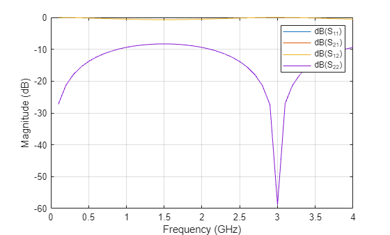
Calculate and plot the S-parameters with the reference impedance of 50.
freq = (1:40)*100e6;
Srf = sparameters(tx,freq,50);
rfplot(Srf)
Calculate the characteristic impedance.
Zc_rf = getZ0(tx)
Zc_rf =
75.0279
EM Modeling
Input the microstrip transmission line to the microstripLine object from the RF PCB Toolbox for EM modeling.
tx_em = microstripLine(tx)
tx_em =
  microstripLine with properties:

              Length: 0.0471
               Width: 0.0035
              Height: 0.0016
    GroundPlaneWidth: 0.0175
           Substrate: [1×1 dielectric]
           Conductor: [1×1 metal]
          IsShielded: 0
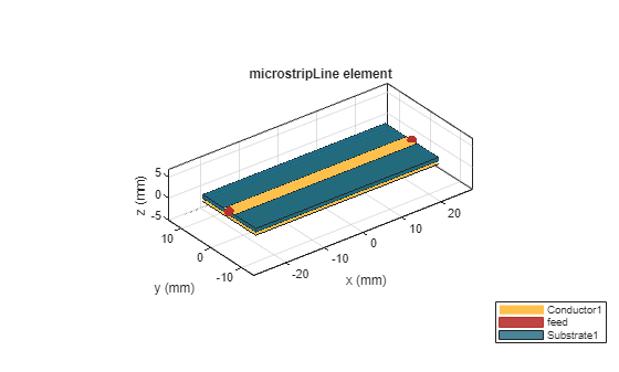
View the suspended microstrip transmission line.
show(tx_em)
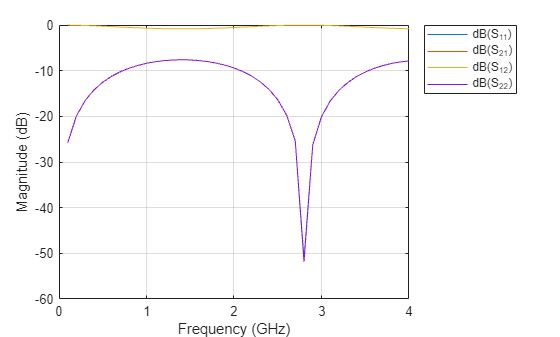
Calculate and plot the S-parameters using EM solver from RF PCB Toolbox.
Sem = sparameters(tx_em,freq,50);
rfplot(Sem)
Zc_em = getZ0(tx_em)
Zc_em =
72.8505 - 0.2106i
Select the dielectric and metal layers for an inverted microstrip transmission line from the dielectric and metal libraries, respectively, of the RF PCB Toolbox™.
dFR4 = dielectric('FR4');
dFR4.Thickness = 3.2e-4;
mCopper = metal('Copper');
Create an inverted microstrip transmission line with a copper conductor and an FR4 substrate at 6 GHz with the line length of 0.5 and the reference impedance of 75. The air to substrate thickness ratio is calculated using:
prototype_behavioral = txlineMicrostrip(Type="Inverted", ...
    DielectricThickness=dFR4.Thickness,EpsilonR=dFR4.EpsilonR, ...
    Height=12.8e-4,LossTangent=dFR4.LossTangent, ...
    SigmaCond=mCopper.Conductivity,Thickness=mCopper.Thickness);
Input the inverted microstrip transmission line to the microstripLine object from the RF PCB Toolbox for EM modeling.
prototype_em = microstripLine(prototype_behavioral);
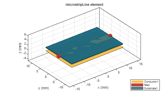
Use the design (Antenna Toolbox) function to design the microstripLine (RF PCB Toolbox) object at 6 GHz with the line length of 0.5 and reference impedance of 75.
tx = design(prototype_em,6e9,'Z0',75,'LineLength',0.5);
View the microstipLine object.
show(tx)
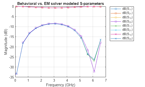
Plot S-Parameters
Calculate and plot the behavioral and electromagnetic (EM) solver modeled S-parameters of the line with the reference impedance of 50. Use the Behavioral name-value argument of the sparameters (RF PCB Toolbox) function to compute the behavioral S-parameters.
freq = (1:5:66)*100e6;
Srf = sparameters(tx,freq,50,'Behavioral',true);
Sem = sparameters(tx,freq,50);
rfplot(Srf,'-s','db')
hold on
rfplot(Sem,'-x','db')
title("Behavioral vs. EM solver modeled S-parameters");
Algorithms
When you set the
StubModeproperty to'Shunt', the 2-port network consists of a stub transmission line that you can terminate with either a short circuit or an open circuit.
Zin is the input impedance of the shunt circuit. The ABCD-parameters for the shunt stub are calculated as:
When you set the
StubModeproperty to'Series', the 2-port network consists of a series transmission line that you can terminate with either a short circuit or an open circuit.
Zin is the input impedance of the series circuit. The ABCD-parameters for the series stub are calculated as:
References
[1] Garg, Ramesh, I. J. Bahl, and Maurizio Bozzi. Microstrip Lines and Slotlines. 3rd ed. Artech House Microwave Library. Boston: Artech House, 2013.
[2] Wadell, Brian C. Transmission Line Design Handbook. The Artech House Microwave Library. Boston: Artech House, 1991.
Version History
Introduced in R2020bSee Also
microstripLine (RF PCB Toolbox) | txlineCoaxial | txlineCPW | txlineParallelPlate | txlineRLCGLine | txlineTwoWire