Simulate Radar Detections of Surface Targets in Clutter
This example shows how to simulate the detection of targets in surface clutter. You will first see how to use a statistical radar model to examine the effect of Doppler separation on detectability, then use terrain data to see how line-of-sight occlusions can be simulated in a radar scenario.
rng defaultDetecting Surface Targets With Clutter Doppler Separation
This section demonstrates how Doppler separation allows moving targets to be detected even when surface reflections are significant. You will configure a radar scenario to simulate a typical side-looking airborne radar that is pointing at a surface target. You will first let the target be stationary, then calculate a velocity vector that separates the target from clutter, and examine the resulting detections.
Stationary Target
Start by creating a radarDataGenerator. Set MountingAngles so that the radar is pointing to the right of the platform (a -90 degree mounting yaw angle) and pointing down at 15 degrees (a 15 degree depression angle). Use a frequency of 1 GHz, 100 meter range resolution, a 5 kHz PRF, and 128 pulses. The beam is symmetric with a 4 degree two-sided beamwidth in azimuth and elevation.
mountingYPR = [-90 15 0];
fc = 1e9;
rangeRes = 100;
prf = 5e3;
numPulses = 128;
beamwidth = 4;
Use the PRF and number of pulses specification to calculate the nominal Doppler and range-rate resolution.
dopRes = prf/numPulses;
lambda = freq2wavelen(fc);
rangeRateRes = dop2speed(dopRes,lambda)/2;
Pulse-Doppler radars have both range and range-rate ambiguities. Calculate the unambiguous range and radial speed.
unambRange = time2range(1/prf);
unambRadialSpd = dop2speed(prf/4,lambda);
Construct the radarDataGenerator. Let the sensor index equal 1 and disable scanning functionality. The radar will update once per coherent processing interval (CPI). Configure the operating mode to be monostatic, with detections output in scenario coordinates. Enable elevation angle measurements, range-rate measurements, and the range and range-rate ambiguities. Disable false alarms and detection noise so that the effect of Doppler separation can be seen clearly. Lastly, set the reference target used to compute the loop gain to a 0 dBsm target at 20 km range, with a detection probability of 90%.
cpiTime = numPulses/prf;
rdr = radarDataGenerator(1,'No scanning','UpdateRate',1/cpiTime,'MountingAngles',mountingYPR,...
    'DetectionMode','Monostatic','TargetReportFormat','Detections','DetectionCoordinates','Scenario',...
    'HasINS',true,'HasElevation',true,'HasFalseAlarms',false,'HasNoise',false,'HasRangeRate',true,...
    'HasRangeAmbiguities',true,'HasRangeRateAmbiguities',true,'MaxUnambiguousRadialSpeed',unambRadialSpd,...
    'MaxUnambiguousRange',unambRange,'CenterFrequency',fc,'FieldOfView',beamwidth,...
    'AzimuthResolution',beamwidth,'ElevationResolution',beamwidth,'RangeResolution',rangeRes,'RangeRateResolution',rangeRateRes,...
    'ReferenceRange',20e3,'ReferenceRCS',0,'DetectionProbability',0.9);
Create the scenario, setting the update rate to 0 to let the update intervals be derived from sensors in the scene.
scene = radarScenario('UpdateRate',0,'IsEarthCentered',false);
The landSurface scenario method is used to define properties of regions of the scenario surface. You will use it here to specify an unbounded homogeneous surface with an associated reflectivity model. Use a constant-gamma reflectivity with a gamma value appropriate for flatland, which can be found with the surfacegamma function. surfaceReflectivity is used to create the land reflectivity model that will be associated with the scenario surface through the RadarReflectivity property.
gammaDB = surfacegamma('Flatland');
refl = surfaceReflectivity('Land','Model','ConstantGamma','Gamma',gammaDB);
landSurface(scene,'RadarReflectivity',refl);
Now define the radar platform. The platform will start 4 km above the origin, and fly in the +Y direction at 200 m/s. Set the platform orientation such that the platform-frame X is aligned with the direction of motion. With the mounting angles specified on the radar, this means the radar will be pointed in the +X direction.
altitude = 4e3;
rdrpos = [0 0 altitude];
rdrspd = 200;
rdrtraj = kinematicTrajectory('Position',rdrpos,'Velocity',[0 rdrspd 0],'Orientation',rotz(90).');
rdrplat = platform(scene,'Sensors',rdr,'Trajectory',rdrtraj);
The figure below shows a visualization of this scenario geometry, including the homogeneous land surface.
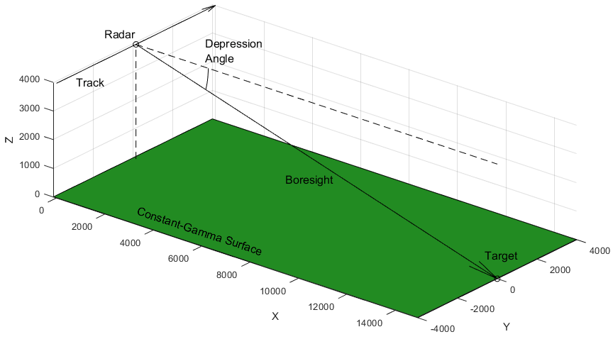
Place the target on the surface along the radar boresight direction. The required ground range can be found from the radar altitude and depression angle.
gndrng = altitude/tand(mountingYPR(2));
tgtpos = [gndrng 0 0];
Choose the target RCS such that the return signal would be buried in clutter without any Doppler separation. Do this by calculating an approximate RCS of clutter in a broadside range-Doppler resolution cell, and then setting the target RCS to one quarter of that. The reflectivity model defined previously can be used to get the NRCS, and the approximate area of the resolution cell can be found with the provided helper function. Express the RCS in dBsm.
clutterCellNRCS = refl(mountingYPR(2),fc);
clutterCellArea = helperBroadsideResCellArea(rangeRes,rangeRateRes,gndrng,mountingYPR(2),rdrspd);
clutterCellRCS = clutterCellNRCS*clutterCellArea;
tgtrcs = clutterCellRCS/4;
tgtrcs = 10*log10(tgtrcs);
Calculate the expected SNR of the target for later comparison to the SNR of the resulting detections. The RadarLoopGain property of the radar gives the relationship between target RCS, range, and SNR.
tgtrng = sqrt(altitude^2 + gndrng^2);
tgtsnr =  tgtrcs - 40*log10(tgtrng) + rdr.RadarLoopGain
tgtsnr =
32.3399
Use the scenario platform method to create a stationary target platform and add it to the scene. The rcsSignature class can be used to define a constant-RCS signature by using a scalar RCS value for the Pattern property.
tgtplat = platform(scene,'Position',tgtpos,'Signatures',rcsSignature('Pattern',tgtrcs));
Now, use the scenario clutterGenerator method to construct a clutter generator and enable clutter generation for your radar. The Resolution property defines the nominal spacing of clutter patches. Set this to be 1/5th of the range resolution to get multiple clutter patches per range gate. Set the range limit to 20 km to encompass the entire beam. UseBeam indicates if clutter generation should be performed automatically for the mainlobe of the antenna pattern, or for the field of view of a radarDataGenerator, as defined by the FieldOfView property.
clut = clutterGenerator(scene,rdr,'Resolution',rangeRes/5,'RangeLimit',20e3,'UseBeam',true);
Now the simulation is fully configured. Run the simulation for a single frame, collecting detections from the radar you constructed. This can be done by calling the scenario detect method.
dets = detect(scene);
Examine one of these detections.
dets{1}ans =
objectDetection with properties:
Time: 0
Measurement: [6×1 double]
MeasurementNoise: [6×6 double]
SensorIndex: 1
ObjectClassID: 0
ObjectClassParameters: []
MeasurementParameters: [1×1 struct]
ObjectAttributes: {[1×1 struct]}
Each objectDetection contains information about a detection made in a particular resolution cell. The Measurement property will give the position and velocity of the detection in scenario coordinates, and SensorIndex refers to the index assigned to the radarDataGenerator upon construction. Useful metadata can be found by inspecting the contents of the ObjectAttributes property.
dets{1}.ObjectAttributes{1}ans = struct with fields:
TargetIndex: 14
SNR: 38.8084
The TargetIndex field gives the index of the target that generated the detection. If multiple targets fall inside the same resolution cell, this will be the index of the target in that cell with the greatest signal power. This index corresponds to the PlatformID property of the target platforms. This ID is assigned automatically upon creating a platform, and increments by 1 with each new platform. When clutter is being simulated, the target index may exceed the number of platforms added to the scenario, which indicates that the detection came from a resolution cell where clutter return was dominant.
The low SNR of the first detection shown above is due to the sorted output from the radarDataGenerator. Within the field of view of the radar, clutter power in cells on the low side of the range swath are smaller than those at the center, near the intersection of the radar boresight with the ground plane, where the target platform is located. Plot the SNR across all clutter detections to verify the clutter power statistics are as expected.
helperPlotDetectionSNR(dets)
title('Clutter Detection SNR')
The distinct lines correspond to different Doppler bins. The mean SNR of detections in the 0 Hz Doppler bin (corresponding to the higher trend line) is about 6 dB higher than the target SNR, as expected.
Since the target platform of interest was the second platform added to the scene, it will have an ID of 2.
tgtplat.PlatformID
ans =
2
This can be used to find the object detection corresponding to the target platform, if the target was detected. Get the TargetIndex across all detections and see if any correspond to the target platform ID.
tgtidx = cellfun(@(t) t.ObjectAttributes{1}.TargetIndex,dets);
tgtdet = dets(tgtidx == tgtplat.PlatformID);
detectedPlatform = ~isempty(tgtdet)
detectedPlatform = logical
0
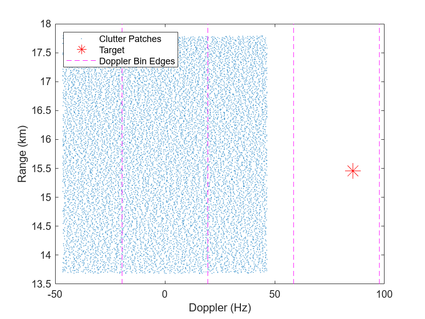
In this scenario, the target platform was not detected because the target return signal fell in the same resolution cell as clutter return. Use the provided helper function to plot a visualization of the target and clutter patches in range-Doppler space with an overlay of the boundaries of the Doppler resolution cells.
helperPlotRangeDoppler(clut,rdrplat,tgtplat,lambda,prf,dopRes)

Since the target was placed on the surface along the antenna boresight and is stationary, it appears at the same point in range-Doppler space as the centroid of the mainlobe clutter return, and is undetectable.
Moving Target
Now you will calculate a velocity vector for the target so it moves along the surface towards the radar (in the -X direction) at a speed such that the return signal will fall outside of the clutter return in Doppler.
First calculate the total range-rate spread of the mainlobe clutter return. This equation is valid for broadside clutter, where the antenna boresight vector is perpendicular to the radar velocity.
clutSpread = 2*rdrspd*sind(beamwidth/2);
Calculate the required closing rate such that the target is one Doppler resolution cell outside of the mainlobe clutter return. Also calculate the total required speed, which can be found by dividing by the magnitude of the X component of the line of sight to the radar position.
los = (rdrpos - tgtpos)/tgtrng;
tgtClosingRate = clutSpread/2 + rangeRateRes;
tgtspd = tgtClosingRate/abs(los(1));
Set the target velocity by accessing the platform trajectory, which is a kinematicTrajectory by default.
tgtplat.Trajectory.Velocity = [-tgtspd 0 0];
Run the simulation for another frame.
dets = detect(scene);
Once again, get the target index for each detection and search for one that corresponds to the target platform.
tgtidx = cellfun(@(t) t.ObjectAttributes{1}.TargetIndex,dets);
tgtdet = dets(tgtidx == tgtplat.PlatformID);
detectedPlatform = ~isempty(tgtdet)
detectedPlatform = logical
1
This time, the target was detected. Inspect the measured position and object attributes of the target detection.
if detectedPlatform
    tgtdet{1}.Measurement(1:3)
    tgtdet{1}.ObjectAttributes{:}
end
ans = 3×1
104 ×

     1.4928
     0.0000
    -0.0000
ans = struct with fields:
    TargetIndex: 2
            SNR: 32.3399
The measured target position is accurate to within a few meters, and the reported SNR is as found earlier via the radar loop gain.
View the returns in range-Doppler space.
helperPlotRangeDoppler(clut,rdrplat,tgtplat,lambda,prf,dopRes)
The target return has a Doppler frequency that is one Doppler resolution cell greater than the maximum Doppler of the mainlobe clutter return. Despite the small RCS of the target relative to clutter, it was detectable thanks to Doppler separation.
Detecting Surface Targets in the Presence of Terrain
Terrain Clutter and Occlusions
In this section, you will again construct a radar scenario and examine the detectability of a target in clutter. This time you will use terrain data to place the target on the surface, generate clutter returns, and simulate line-of-sight occlusions between the radar and target.
Start by loading the sample terrain data. This contains the variables terrain and boundary, which will be passed to the landSurface method.
load MountainousTerrain.matCreate the scenario as before. Use the landSurface method to define a rectangular region of terrain by specifying a matrix of height samples and a boundary for the region in two-point form.
scene = radarScenario('UpdateRate',0,'IsEarthCentered',false);
srf = landSurface(scene,'RadarReflectivity',refl,'Terrain',terrain,'Boundary',boundary);
The terrain data covers a region of about 23 km in the X direction and 17 km in the Y direction. This can be seen by inspecting the Boundary property.
srf.Boundary
ans = 2×2
104 ×

          0    2.2920
    -0.8544    0.8544
The radar will again be placed above the origin while viewing a target platform that is moving along the surface towards the radar from the +X direction. Re-create the radar platform, this time using the height method of the surface object to place the radar above the surface at the same altitude used previously.
rdrpos(3) = height(srf,rdrpos) + altitude;
rdrtraj = kinematicTrajectory('Position',rdrpos,'Velocity',[0 rdrspd 0],'Orientation',rotz(90).');
rdrplat = platform(scene,'Sensors',rdr,'Trajectory',rdrtraj);
Re-create the target platform, using the height method to place the target platform on the surface.
tgtpos(3) = height(srf,tgtpos);
tgttraj = kinematicTrajectory('Position',tgtpos,'Velocity',[-tgtspd 0 0]);
tgtplat = platform(scene,'Trajectory',tgttraj,'Signatures',rcsSignature('Pattern',tgtrcs));
Enable clutter generation. This time, since terrain data is being used, the Resolution property is not relevant. Clutter patches will correspond to facets of the terrain data.
clut = clutterGenerator(scene,rdr,'RangeLimit',20e3,'UseBeam',true);
The actual spacing of clutter patches in the X and Y directions can be found by dividing the extent of the surface in each direction by the number of height samples. Note that the X and Y directions are defined for the matrix of height sampled following the meshgrid convention, where the first dimension of the matrix (columns) corresponds to Y and the second dimension (rows) to X.
terrainClutterSpacing = diff(boundary,1,2)./flip(size(terrain)).'
terrainClutterSpacing = 2×1

    29.9608
    25.6188
The terrain data is sampled at 25 to 30 meter resolution, which is sufficient to yield a few clutter patches per resolution cell.
Collect one frame of detections.
dets = detect(scene);
Since the target is moving with the same velocity vector as before, a detection of the target platform might be expected. Plot the clutter patches and target in range-Doppler space again to verify.
helperPlotRangeDoppler(clut,rdrplat,tgtplat,lambda,prf,dopRes)
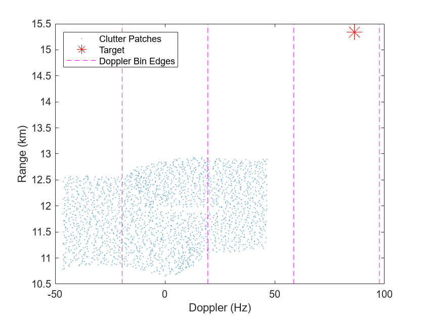
Notice that this time, the target is separated from clutter in both range and Doppler. Notice also that the clutter return is closer in range than in the flat-surface case by about 3 km. The overall extent of clutter in Doppler is the same since that depends only on beamwidth, not the shape of the surface.
Check to see if an object detection corresponding to the target platform was generated.
tgtidx = cellfun(@(t) t.ObjectAttributes{1}.TargetIndex,dets);
tgtdet = dets(tgtidx == tgtplat.PlatformID);
detectedPlatform = ~isempty(tgtdet)
detectedPlatform = logical
0
The target was not detected. Plot the scenario overview to see why, adjusting the view so the effect of terrain can be seen more easily.
helperPlotClutterScenario(scene)
set(gca,'view',[-115 22])
The same geometry parameters were used here as in the homogeneous surface scenario. The target still lies directly along the antenna boresight, but the mainlobe intersects a region of terrain that is at a lower range than the target. The target is thus occluded by the terrain and is not detectable. The occlusion of the LOS to the target can be checked explicitly by using the occlusion method on the surface object. This method will take two points as input and indicate whether or not the LOS between them is occluded by the surface. The platform positions can be passed in directly.
occluded = occlusion(srf,rdrplat.Position,tgtplat.Position)
occluded = logical
   1
This verifies the observation from the scenario overview plot that the target is occluded from the radar by the terrain.
Surface objects in the scenario are managed by a surface manager, which can be accessed through the SurfaceManager property of the scenario. Inspect this property.
scene.SurfaceManager
ans =
  SurfaceManager with properties:

    EnableMultipath: 0
       UseOcclusion: 1
           Surfaces: [1×1 radar.scenario.LandSurface]
The manager contains a read-only vector of surface objects present in the scenario, and a logical indicator that can be used to enable/disable line-of-sight occlusions by surface features. Try disabling this now, collecting detections for another frame, and checking for a target platform detection.
scene.SurfaceManager.UseOcclusion = false;
dets = detect(scene);
tgtidx = cellfun(@(t) t.ObjectAttributes{1}.TargetIndex,dets);
tgtdet = dets(tgtidx == tgtplat.PlatformID);
detectedPlatform = ~isempty(tgtdet)
detectedPlatform = logical
1
With surface occlusion disabled, the platform is detectable.
Simulate Multiple Surface Targets
In this next section, you will place multiple platforms at random positions on the surface and simulate detections while observing terrain occlusions, included automatically as part of the scenario detect method. Clutter detections will not be simulated here in order to simplify the simulation and highlight the terrain occlusion effects (that is, assume all targets are detectable given that they are visible to the radar). To include interference from clutter, the clutterGenerator method could be used as before, though the targets would need to be in motion or have large RCS signatures to be detectable.
Re-create the scenario, using the same terrain data.
scene = radarScenario('UpdateRate',0,'IsEarthCentered',false);
srf = landSurface(scene,'RadarReflectivity',refl,'Terrain',terrain,'Boundary',boundary);
Release the radar object so that it may be reconfigured. Using the same field of view, enable electronic scanning over 90 degrees in azimuth and 16 degrees in elevation in order to cover most of the surface. All targets will be illuminated over the course of a full scan.
release(rdr)
rdr.ScanMode = 'Electronic';
rdr.ElectronicAzimuthLimits = [-45 45];
rdr.ElectronicElevationLimits = [-8 8];
Modify the trajectory created above to place the radar platform at one corner of the loaded terrain data. The same straight-line trajectory will be re-used. Set the scenario stop time as needed to give the radar time to travel from one end of the terrain to the other, in the Y direction. This will allow for the line of sight to some targets to transition between occluded and unoccluded.
rdrtraj.Position(2) = boundary(2,1);
rdrplat = platform(scene,'Sensors',rdr,'Trajectory',rdrtraj);
scene.StopTime = diff(srf.Boundary(2,:))/rdrspd;
Place down targets at random positions on the surface. The minimum value of the position in the X direction is chosen so that all targets will fall within the field of view of the radar at some point during the scan. The targets are uniformly distributed in the Y direction, and the height method is again used to place them on the surface.
numtgt = 14;
tgtpos(1,1:numtgt) = 1e4 + rand(1,numtgt)*(srf.Boundary(1,2) - 1e4);
tgtpos(2,:) = srf.Boundary(2,1) + rand(1,numtgt)*diff(srf.Boundary(2,:),1,2);
tgtpos(3,:) = height(srf,tgtpos);
for ind = 1:numtgt
   platform(scene,'Position',tgtpos(:,ind).');
end
Each iteration of the simulation loop constitutes one scan position. The second output from the scenario detect method, config, returns some information on the configuration of the radarDataGenerator that produced the detections. The IsScanDone field is a logical scalar that indicates if the radar was on its final scan position on the last call to detect. The detections from each scan position will be saved and when the scan pattern is completed, a visualization of the occlusion states and resulting detections will be plotted.
figure;
p = get(gcf,'Position');
set(gcf,'Position',[p(1:2) 2*p(3:4)])
fullScanDets = [];
while advance(scene)
    [dets,config] = detect(scene);
    fullScanDets = [fullScanDets; dets];
    if config.IsScanDone
        helperPlotOcclusions(scene,fullScanDets)
        drawnow
        fullScanDets = [];
    end
end
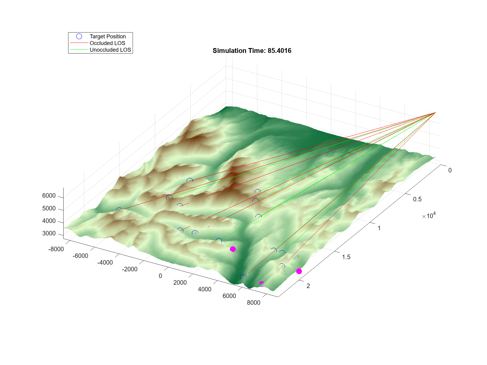
The below gif shows the resulting animation. Since all visible targets are illuminated at some point during a complete scan, detections are made whenever a target is visible, while targets with occluded lines of sight are not detected.
Conclusion
In this example, you saw how to configure a radarScenario and radarDataGenerator to simulate detections of a surface target in clutter. You used a ClutterGenerator with a simple homogeneous surface to examine the effect of Doppler separation, then used terrain data to simulate the effect of line-of-sight occlusions on detectability.
Supporting Functions
helperBroadsideResCellArea
function A = helperBroadsideResCellArea( rangeRes,rangeRateRes,groundRange,graze,speed )
% Calculate the approximate area of a broadside range-Doppler resolution
% cell

% Ground range resolution
groundRangeRes = rangeRes/cosd(graze);

% Broadside angular variation corresponding to Doppler resolution
dtheta = 2*asin(rangeRateRes/(2*speed));

% Multiply by ground range to get cross-range extent
crossRangeWidth = groundRange*dtheta;

% Cell area
A = crossRangeWidth*groundRangeRes;

end
helperPlotDetectionSNR
function helperPlotDetectionSNR( dets )
% Plot the SNR of a set of objectDetections

detsnr = cellfun(@(t) t.ObjectAttributes{1}.SNR,dets);
plot(detsnr,'.')
grid on
xlabel('Detection Index')
ylabel('SNR (dB)')

end
helperPlotRangeDoppler
function helperPlotRangeDoppler( clut,rdrplat,tgtplat,lambda,prf,dopRes )
% Plot the range-Doppler truth of clutter patches and a target, along with
% an indication of the edges of the Doppler resolution cells.

% Get range and Doppler to target
los = rdrplat.Position - tgtplat.Position;
tgtRange = norm(los);
los = los/tgtRange;
tgtDoppler = 2/lambda*sum((tgtplat.Trajectory.Velocity-rdrplat.Trajectory.Velocity).*los);

% Get range and Doppler to clutter patches
patches = clut.LastPatchData.Centers;
los = patches - rdrplat.Position(:);
clutterRange = sqrt(sum(los.^2,1));
los = los ./ clutterRange;
clutterDoppler = 2/lambda*sum(rdrplat.Trajectory.Velocity(:).*los,1);

% Plot clutter and target in range-Doppler space
plot(clutterDoppler,clutterRange/1e3,'.','markersize',.1)
hold on
plot(tgtDoppler,tgtRange/1e3,'*r','markersize',15)

% Plot the Doppler bin edges
xl = xlim;
yl = ylim;
dopBins = -prf/2:dopRes:(prf/2-dopRes);
dopBinEdges = [dopBins(1)-dopRes/2, dopBins+dopRes/2];
dopBinEdges = dopBinEdges(dopBinEdges >= xl(1) & dopBinEdges <= xl(2));
line([1 1].'*dopBinEdges,repmat(yl,numel(dopBinEdges),1).','color','magenta','linestyle','--')
hold off

legend('Clutter Patches','Target','Doppler Bin Edges','Location','northwest')

xlabel('Doppler (Hz)')
ylabel('Range (km)')

end
helperPlotOcclusions
function helperPlotOcclusions( scene,dets )
% Plot the scenario surface along with target and radar positions and the
% lines of sight between them, color coding to indicate the occlusion state
% of each line of sight. Also plot the position of any detections.

% Plot the surface
helperPlotScenarioSurface(scene.SurfaceManager.Surfaces(1))
hold on

% Find radar platform and get current position
plats = [scene.Platforms{:}];
hasSensor = ~cellfun(@isempty,{plats.Sensors});
rdrplat = plats(find(hasSensor,1));
rdrpos = rdrplat.sensorPosition(1);

% Target platforms
tgtplats = plats(plats ~= rdrplat);

for ind = 1:numel(tgtplats) % for each target

    % Position of current target
    tgtpos = tgtplats(ind).Position;

    hndls(1) = plot3(tgtpos(1),tgtpos(2),tgtpos(3),'oblue','MarkerSize',10);

    % Get occlusion state by querying the scenario surface manager
    occ = occlusion(scene.SurfaceManager,rdrpos,tgtpos,scene.SimulationTime);

    % Plot color-coded line of sight
    if occ
        hndls(2) = line([rdrpos(1) tgtpos(1)],[rdrpos(2) tgtpos(2)],[rdrpos(3) tgtpos(3)],'color','red');
    else
        hndls(3) = line([rdrpos(1) tgtpos(1)],[rdrpos(2) tgtpos(2)],[rdrpos(3) tgtpos(3)],'color','green');
    end

end

% Keep only detections originating from target platforms
tgtidx = cellfun(@(t) t.ObjectAttributes{1}.TargetIndex,dets);
targetDetection = any(tgtidx == [plats.PlatformID],2);
dets = dets(targetDetection);

% Plot detections
if ~isempty(dets)
    detpos = cell2mat(cellfun(@(t) t.Measurement(1:3),dets.','UniformOutput',0));
    plot3(detpos(1,:),detpos(2,:),detpos(3,:),'omagenta','MarkerSize',9,'MarkerFaceColor','magenta');
end

hold off
legendstr = ["Target Position" "Occluded LOS" "Unoccluded LOS" "Detection Positions"];
I = ishghandle(hndls);
hndls = hndls(I);
legendstr = legendstr(I);
legend(hndls,legendstr,'Location','Northwest');
title(sprintf('Simulation Time: %.4f',scene.SimulationTime))
view([120 28])

end