Simulate an Automotive 4D Imaging MIMO Radar

This example shows how to simulate a 4D imaging MIMO radar for automotive applications using radarTransceiver. You will learn how to generate I/Q data with the radar in a simulated environment. The I/Q data will be processed to generate a point cloud of radar detections.

Model a MIMO Radar Transceiver

Use radarTransceiver to create a signal-level radar transceiver model for an FMCW automotive MIMO radar. You will use this model to simulate baseband I/Q signals at the output of the radar receiver.

rng default; % Set random seed for reproducible results
xcvrMIMO = radarTransceiver();

% Create FMCW waveform
rgRes = 0.5; % meters
rgMax = 150; % meters
sweepBW = rangeres2bw(rgRes); % Hz
Fs = sweepBW;

% Set the sweep time to at least twice the max range time to avoid power
% loss at the max range extent. Longer sweep times give higher
% signal-to-noise ratios (SNRs) at greater ranges, but at the cost of
% maximum ambiguous velocity
sweepTime = 4*range2time(rgMax); % s
Ncp = 512; % Number of chirps

wfm = phased.FMCWWaveform( ...
    'SweepBandwidth',sweepBW, ...
    'SweepTime',sweepTime, ...
    'SampleRate',Fs);
xcvrMIMO.Waveform = wfm;
xcvrMIMO.Receiver.SampleRate = Fs;
xcvrMIMO.NumRepetitions = Ncp;

% Set receiver gain and noise level
xcvrMIMO.Receiver.NoiseFigure = 12;

disp(xcvrMIMO);

  radarTransceiver with properties:

                Waveform: [1×1 phased.FMCWWaveform]
             Transmitter: [1×1 phased.Transmitter]
         TransmitAntenna: [1×1 phased.Radiator]
          ReceiveAntenna: [1×1 phased.Collector]
                Receiver: [1×1 phased.ReceiverPreamp]
      MechanicalScanMode: 'None'
      ElectronicScanMode: 'None'
        MountingLocation: [0 0 0]
          MountingAngles: [0 0 0]
    NumRepetitionsSource: 'Property'
          NumRepetitions: 512
       RangeLimitsSource: 'Property'
             RangeLimits: [0 Inf]
         RangeOutputPort: false
          TimeOutputPort: false

Define MIMO Transmit and Receive Arrays

MIMO radar is widely used for automotive radar applications due to its ability to realize small angular resolutions in azimuth and elevation within a small package. For high-resolution 4D radar, beamwidths in azimuth and elevation less than 2 degrees are desired. Compute the number of array elements that would be needed to realize a 2 degree beamwidth for a linear array.

fc = 77e9; % Hz
lambda = freq2wavelen(fc); % m

% Compute array aperture
d = beamwidth2ap(2,lambda,0.8859);

% Compute number of array elements required for half-wavelength spacing
disp(2*d/lambda)

   50.7583

If conventional arrays with elements at half-wavelength spacing were used, an array with 50 elements would be required to realize a resolution of 2 degree in azimuth, and another 50 elements would be needed if a similar resolution was desired in elevation. If a uniform rectangular array (URA) was to be used, a total of 50 x 50 = 2500 elements would be required.

Instead, let's define a virtual array which is composed of separate transmit and receive antenna arrays. Create a uniform linear array (ULA) for the transmit antenna with half-wavelength spacing and a rectangular receive array which does not maintain a half-wavelength spacing in the azimuth dimension.

% Define transmit ULA element positions
Ntx = 10;
txPos = [ ...
    0:Ntx-1; ...        % y positions
    zeros(1,Ntx)];      % z positions
txPos = sortrows(txPos',[2 1])';

% Define receive URA element positions
Naz = 5; % Azimuth array is number of transmit elements times half-wavelength spacing
Nel = 50; % Elevation array at half-wavelength spacing

[yPos,zPos] = meshgrid((0:Naz-1)*Ntx,0:Nel-1);
rxPos = [yPos(:) zPos(:)]';

% Sort the rows to allow the virtual array elements to be assembled later
rxPos = sortrows(rxPos',[2 1])';

Use helperVirtualArray to generate the transmit and receive arrays and the corresponding virtual array element positions.

[txArray,rxArray,vxPos] = helperVirtualArray(txPos,rxPos,lambda);
helperViewArrays(txPos,rxPos,vxPos);

A virtual array with 2500 elements is created by using a 10 element transmit array and a 5 x 50 = 250 element receive array. This results in a significant reduction in the number of required elements and hardware complexity. For more information on how a virtual array is defined, see the Increasing Angular Resolution with Virtual Arrays example.

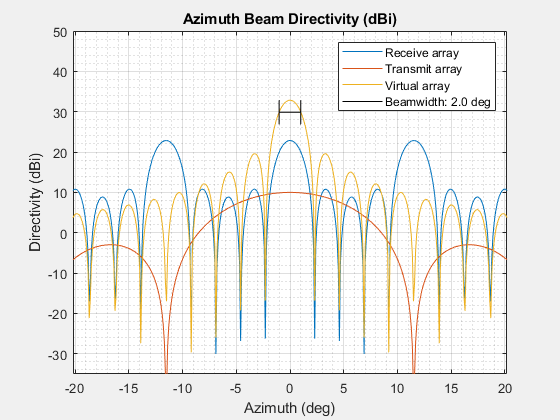
Use helperPlotDirectivities to plot the directivities for the transmit, receive, and virtual arrays in azimuth and elevation.

bwAz = helperPlotDirectivities(txArray,rxArray,fc);

bwEl = helperPlotDirectivities(txArray,rxArray,fc,'Elevation');

% Compute the total number of elements used
disp(getNumElements(txArray) + getNumElements(rxArray))

   260

We realized a 2 degree beamwidth in azimuth and elevation by using 260 elements instead of the 2500 elements that would have been needed for a full rectangular array.

Attach the transmit and receive arrays used to define the virtual array to the MIMO radar model.

% Attach transmit and receive arrays
xcvrMIMO.TransmitAntenna.Sensor = txArray;
xcvrMIMO.TransmitAntenna.OperatingFrequency = fc;
xcvrMIMO.ReceiveAntenna.Sensor = rxArray;
xcvrMIMO.ReceiveAntenna.OperatingFrequency = fc;

% Configure transmitter for MIMO mode
xcvrMIMO.ElectronicScanMode = 'Custom';
xcvrMIMO.TransmitAntenna.WeightsInputPort = true;

% Set transmitter gain and power level
xcvrMIMO.Transmitter.PeakPower = db2pow(10);

Define MIMO DDMA Waveform

An essential characteristic of any MIMO radar implementation is a waveform that maintains orthogonality along all the transmit antennas. This orthogonality is often realized by encoding the transmitted waveforms in time, frequency, or code domains. Maintaining this orthogonality across the transmit antennas is essential in order to assemble the virtual array used by the MIMO radar as will be demonstrated later in the Signal Processing section of this example. Time Division Multiple Access (TDMA) is a common technique used to maintain orthogonality in the time domain. TDMA only transmits from one antenna element at any given time. Only using one transmit element at a time maintains the needed orthogonality but at the cost of reducing the total transmit power and decreasing the maximum unambiguous velocity of the radar. For more information on TDMA MIMO radar, see the Increasing Angular Resolution with Virtual Arrays example.

Instead of maintaining orthogonality in the time domain, new techniques using the frequency and code domains have been proposed. One such technique, Doppler Division Multiple Access (DDMA) MIMO maintains orthogonality in the frequency domain by shifting the waveforms transmitted by each antenna in Doppler. The motivation of this conventional DDMA scheme is to separate transmit signals from the Ntx transmit antennas into Ntx Doppler frequency subbands at the receiver. This is realized by DDMA MIMO weights which modulate each transmit antenna's signal into its own Doppler frequency subband. A drawback of this technique is that the maximum ambiguous velocity is still reduced by the number of transmit antennas due to the Ntx peaks from the transmitted signals spread across the Doppler space. An adaptation of the conventional DDMA MIMO which introduces an unused region of Doppler without regularly spaced peaks by adding virtual transmit elements to the array is used here. This enables the maximum ambiguous velocity of the radar's waveform to be maintained. [1], [2]

Create a DDMA waveform for the MIMO radar that assigns a unique Doppler offset to each of the transmit elements so that each element will transmit the same FMCW waveform, but with a unique offset in Doppler. Generate the Doppler offsets uniformly across the Doppler space for the 10 transmit antennas and 2 virtual antennas. This will assign two Doppler offsets to unused virtual transmit elements. These unused Doppler offsets will enable Doppler ambiguities to be unwrapped, preventing a reduction in the maximum ambiguous velocity of the MIMO radar.

% Define an (Ntx + Nvtx)-by-Ncp DFT matrix where Nvtx > 0 so that Nvtx
% Doppler bins are unused
Nvtx = 2;

[dopOffsets,Nv] = DDMAOffsets(Ntx,Nvtx);
% Recompute Ncp so that it is a multiple of Nv. This is important for
% recovering transmitted signal.
Ncp = ceil(Ncp/Nv)*Nv;
xcvrMIMO.NumRepetitions = Ncp;

% Select Ntx consecutive Doppler offsets for the DDMA weights
wDDMA = dopMatrix(dopOffsets(1:Ntx),Ncp);
% Show the DDMA Doppler offsets
plotDDMAOffsets(dopOffsets,Ntx);

The FMCW waveform transmitted on each of the 10 elements will have a Doppler offset corresponding to each of the vectors in the previous figure. The DDMA weights have been chosen so that they are centered on zero Doppler. In the preceding figure, Doppler is represented as degrees on the unit circle by normalizing the Doppler shift frequencies from [-PRF/2,PRF/2] by PRF/2$\pi$. The Doppler shift applied to transmit element is -135 degrees.

Simulate Radar Data Cube

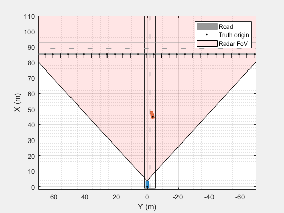
Use helperCreateOverpassScenario to create a drivingScenario that includes a highway overpass along with a vehicle merging into the lane in front of the ego vehicle. Mount the MIMO radar to the front of the ego vehicle as a forward-looking radar.

% Create drivingScenario
[scenario, egoVehicle] = helperCreateOverpassScenario();

% Mount MIMO radar as forward-looking radar on the ego vehicle
xcvrMIMO.MountingLocation(1) = egoVehicle.Length-egoVehicle.RearOverhang;
xcvrMIMO.MountingLocation(3) = 0.5;
xcvrMIMO.MountingAngles(2) = -5; % Pitch radar upward, away from the road's surface

% Define a coverage configuration structure for use with helperSetupDisplay
fov = [85 25]; % [azimuth elevation] degrees
% rgRes = bw2rangeres(wfm.SweepBandwidth); % meters
covCfg = struct( ...
    'SensorLocation',xcvrMIMO.MountingLocation(1:2), ...
    'MaxRange',rgMax, ...
    'Yaw',xcvrMIMO.MountingAngles(1), ...
    'FieldOfView',fov, ...
    'AzimuthResolution',bwAz, ...
    'ElevationResolution',bwEl, ...
    'RangeResolution',rgRes);

% Plot scenario
bep = helperSetupDisplay(egoVehicle,covCfg);
delete(bep.Plotters(end));
axis(bep.Parent,[-2 110 70*[-1 1]]);

Use helperPosesToPaths to generate propagation path structs from the scenario.

% Convert target poses to path structs
tposes = targetPoses(egoVehicle);
paths = helperPosesToPaths(tposes,xcvrMIMO,scenario,covCfg);

Use the MIMO radar model to generate a Radar Data Cube from the propagation path structs. The radar data cube contains the I/Q signals corresponding to the complex-valued baseband samples collected at the output of the radar's receiver.

time = scenario.SimulationTime;
datacube = xcvrMIMO(paths,time,conj(wDDMA));

Process MIMO Radar Data Cube

Range, Doppler, beamforming, and detection processing need to be applied to the data cube to extract the detection point cloud. For DDMA MIMO, the range and Doppler processing and CFAR detection are applied first so that the virtual array elements can be assembled prior to beamforming.

Range and Doppler Processing

Use phased.RangeDopplerResponse to take the 2D FFT along the first and third dimensions of the data cube to transform the fast- and slow-time dimensions of the data cube into range and Doppler bins respectively. Use Hann windows along the fast- and slow-time dimensions to suppress sidelobes in range and Doppler.

wfm = xcvrMIMO.Waveform;
rgdpProc = phased.RangeDopplerResponse( ...
    'RangeMethod','FFT', ...
    'SampleRate',wfm.SampleRate, ...
    'SweepSlope',wfm.SweepBandwidth/wfm.SweepTime, ...
    'DechirpInput',true, ...
    'RangeWindow','Hann', ...
    'DopplerWindow','Hann', ...
    'DopplerOutput','Frequency');
refSig = wfm();
[rgdpCube,rgBins,dpBins] = rgdpProc(datacube,refSig);

% Limit data to ranges of interest
inRg = rgBins>=0 & rgBins<=covCfg.MaxRange;
rgBins = rgBins(inRg);
rgdpCube = rgdpCube(inRg,:,:);
dpBins = -dpBins;

CFAR Detection

Use a constant false-alarm rate (CFAR) detector to identify the locations of the target returns in the range and Doppler processed data cube.

% Compute the power of each cell in the data cube
pwrCube = abs(rgdpCube).^2;

Configure the CFAR detector to exclude the multiple peaks generated in Doppler for each target due to the Doppler offsets applied at each transmit element by the DDMA MIMO waveform.

% CFAR configuration example
%   [++++---o---++++]
%   o: cell under test
%   -: 6 guard cells
%   +: 8 training cells
fpks = Ncp/Nv; % Distance between DDMA peaks
cfar = phased.CFARDetector( ...
    'NumGuardCells',even(ceil(fpks*0.5)), ... % Use 1/2 of space between DDMA Doppler peaks as guard cells
    'ProbabilityFalseAlarm',1e-6, ...
    'NoisePowerOutputPort',true);
cfar.NumTrainingCells = 2*(fpks-cfar.NumGuardCells); % Use remaining space for training

Compute the locations of the target returns in the range and Doppler processed data cube for each receive element.

% Reshape data cube to perform CFAR averaging along the Doppler dimension.
[~,Nrx,Ndp] = size(rgdpCube);
data = reshape(pwrCube,[],Ndp);
[detMtx,nPow] = cfar(data,1:size(data,1));

% Reshape the detection matrix to match the dimensions of the original
% range and Doppler processed data cube.
detMtx = reshape(detMtx,size(pwrCube));

% Compute the signal-to-noise ratio (SNR) for the range-Doppler map.
nPow = reshape(nPow,size(pwrCube));
snrCube = pwrCube./nPow;

% Identify the range and Doppler bins where the same target appears across
% the receive elements in the data cube.
detMtx = squeeze(sum(detMtx,2)); % Count the number of common target returns.

% Plot the range and Doppler map.
prf = 1/xcvrMIMO.Waveform.SweepTime;
helperPlotRangeDopplerDDMA(snrCube,rgBins,dpBins,prf,Ntx,Nv);

A range and Doppler map for one of the receive elements is shown in the previous figure. The returns from the target vehicle merging into the lane in front of the ego vehicle appear at a range of 40 meters from the radar and returns corresponding to the highway overpass are located at approximately 80 meters. There are ten returns modulated in Doppler at the same range for each target corresponding to the ten Doppler offsets applied across each of the ten transmit elements. A gap in Doppler between the first and last transmit element's target returns exists because of the virtual transmit antennas used to compute the DDMA Doppler offsets. If no virtual transmit elements were used, it would be impossible to identify the first and last elements of the transmit array due to the cyclic nature of the Doppler domain.

Remove Doppler Ambiguities

Create a matched filter to identify the location of the first transmit element for each of the target returns locations identified by the CFAR detector.

% Generate Doppler transmit test sequence
dPks = Ncp/Nv; % Number of Doppler bins between modulated DDMA target peaks
mfDDMA = zeros(dPks,Ntx);
mfDDMA(1,:) = 1;
mfDDMA = mfDDMA(:)';

fig = findfig('DDMA Matched Filter'); ax = axes(fig);
stem(ax,mfDDMA);
xlabel(ax,'Doppler bin (k)'); ylabel(ax,'h_k');
title(ax,fig.Name);
grid(ax,'on'); grid(ax,'minor');

Compute the cyclical cross-correlation between the DDMA matched filter and the detection matrix returned by the CFAR detector to find the Doppler bins corresponding to the target returns generated by the waveform from the first transmit element.

% Compute cyclical cross-correlation.
[Nrg,Ndp] = size(detMtx);

% Require the same target to appear across the receive channels.
corrMtx = detMtx>=Nrx*0.8;
corrMtx = ifft( fft(corrMtx,Ndp,2) .* fft(mfDDMA,Ndp,2), Ndp,2);
rdDetMtx = corrMtx>=Ntx*0.95;

% Multiple detection crossings will occur due to the waveform's ambiguity
% function in range and Doppler. Isolate the local maxima for each group of
% detections in the range-Doppler image.
snrDetMtx = squeeze(sum(snrCube,2));
snrDetMtx(~rdDetMtx) = NaN;
rdDetMtx = islocalmax(snrDetMtx,1);

% Identify the range and Doppler bins associated with localized detection
% maxima.
iRD = find(rdDetMtx(:));
[iRgDet,iDpDet] = ind2sub(size(rdDetMtx),iRD);
rgDet = rgBins(iRgDet);

% Show the locations of the unambiguous detections corresponding to the
% signal returns from the first transmit element.
ax = findaxes('Range-Doppler Map'); hold(ax,'on');
p = plot(ax,dpBins(iDpDet)/prf,rgDet,'rd','DisplayName','Unambiguous detections');
legend(p,'Unambiguous detections','Location','southwest');

The previous figure shows the locations of the target returns generated by the first transmit element. The merging target vehicle, located at approximately 40 meters in front of the radar is moving at approximately the same velocity as the ego vehicle, so it should have a Doppler offset of zero degrees. However, because a DDMA Doppler offset is applied to the FMCW waveform transmitted from each transmit element, we should expect this DDMA offset in addition to the Doppler offset due to the velocity difference between the ego vehicle and the target vehicle. The returns from the first transmit element should then include the -135 degrees Doppler offset due to the DDMA modulation applied to that element as well.

Remove DDMA Doppler offset applied to the first transmit element to recover the Doppler offset attributed to the velocity difference between the ego and target vehicles. Compute the range-rate of the target returns from the corrected Doppler offsets.

% Apply Doppler correction for DDMA Doppler shift applied on the first
% transmit element.
fd = (0:Ncp-1)/Ncp-0.5;
f1 = dopOffsets(1);
dpDet = mod(fd(iDpDet)+f1+0.5,1)-0.5;

% Compute unambiguous range-rate of detected Doppler bin
prf = 1/xcvrMIMO.Waveform.SweepTime;
dpDet = dpDet*prf;
rrDet = dop2speed(dpDet,lambda)/2;

% Show the range and range-rate extracted from the detected target returns.
fig = findfig('Range-Doppler Detections'); ax = axes(fig);
plot(ax,rrDet,rgDet,'s');
xlabel(ax,'Range-rate (m/s)'); ylabel('Range (m)');
title(ax,'Range-Doppler Detections');
ax.YDir = 'normal';
grid(ax,'on'); grid(ax,'minor'); ax.Layer = 'top';
axis(ax,[dop2speed(prf/2,lambda)/2*[-1 1] 0 covCfg.MaxRange]);

Virtual MIMO Array Beamspace Processing

Use the location of the target returns detected for the first transmit elements to identify the locations of the target returns from the other nine transmit elements to assemble the virtual elements for the virtual MIMO array for each target detection. The virtual elements correspond to every possible pair of transmit and receive array elements.

% Assemble virtual array elements from range-Doppler detections.
dPks = Ncp/Nv; % Number of Doppler bins between modulated DDMA target peaks
iDpTx = mod(iDpDet(:)-(0:Ntx-1)*dPks-1,Ncp)'+1; % Transmit elements are isolated in Doppler.
iRgTx = repmat(iRgDet,1,Ntx)';

% Plot the locations of the target returns to be extracted for the ten
% transmit elements in the range and Doppler map.
plotTxArrayReturns(rgBins,dpBins,iRgTx,iDpTx,Ntx,prf);

The range and Doppler bins corresponding to the target returns from the ten transmit elements have been recovered for each receive element.

Use the range and Doppler bin locations for each of the transmit elements to assemble the elements of the virtual array for each target detection.

% Extract virtual elements from range-Doppler data cube for each detection.
iTx = sub2ind([size(rgdpCube,3) size(rgdpCube,1)],iDpTx(:),iRgTx(:));
vxTgts = permute(rgdpCube,[2 3 1]); % Nrx x Ntx x Nrg
vxTgts = vxTgts(:,iTx); % Nrx x (Ntx x Ndet)
vxTgts = reshape(vxTgts,Nrx,Ntx,[]); % Nrx x Ntx x Ndet

Perform beamforming by computing a 2D FFT along the elements in the virtual array corresponding to the azimuth and elevation dimensions of the virtual array. Use Hanning windows along the azimuth and elevation dimensions to suppress sidelobes in those directions.

% Apply DDMA Doppler offset correction to the virtual array's targets.
wgts = dopMatrix(dopOffsets(1:Ntx));
vxTgts = vxTgts.*wgts';

% Reshape the virtual array target returns so that the elements
% corresponding the azimuth and elevation dimensions lie along the second
% and third dimensions of the data cube.
vxTgts = permute(vxTgts,[3 2 1]); % Ndet x Ntx x Nrx
vxTgts = reshape(vxTgts,[],Naz*Ntx,Nel); % Ndet x Naz x Nel
% Apply azimuth taper along the azimuth dimension of the data cube.
Nvxaz = size(vxTgts,2);
winAz = hanning(Nvxaz);
vxTgts = reshape(winAz,1,Nvxaz,1).*vxTgts;

% Apply elevation taper along the elevation dimension of the data cube.
Nvxel = size(vxTgts,3);
winEl = hanning(Nvxel);
vxTgts = reshape(winEl,1,1,Nvxel).*vxTgts;

% Apply 2D FFT along azimuth and elevation dimensions of data cube.
azelTgts = fft(fft(conj(vxTgts),Nvxaz,2),Nvxel,3);
azelTgts = fftshift(fftshift(azelTgts,2),3);

% Compute azimuth and elevation bins of beamformed data cube.
azBins = asind(2*((0:size(azelTgts,2)-1)/size(azelTgts,2))-1);
elBins = asind(2*((0:size(azelTgts,3)-1)/size(azelTgts,3))-1);

Use a CFAR detector to estimate the signal-to-noise ratio (SNR) of the detections in the azimuth and elevation beams.

% Estimate signal-to-noise ratio from detection beams
pwrCube = abs(azelTgts).^2;

cfar = phased.CFARDetector( ...
    'NumGuardCells',4, ...
    'NumTrainingCells',16, ...
    'NoisePowerOutputPort',true);

% Reshape data to perform CFAR averaging for each detection across azimuth
% and elevation bins.
pwrCube = permute(pwrCube,[2 1 3]); % Naz x Ndet x Nel
[~,nPow] = cfar(pwrCube(:,:),1:size(pwrCube,1));
nPow = reshape(nPow,size(pwrCube));
pwrCube = permute(pwrCube,[2 1 3]); % Ndet x Naz x Nel
nPow = permute(nPow,[2 1 3]); % Ndet x Naz x Nel
snrCube = pwrCube./nPow;
snrdB = pow2db(snrCube);

Use the SNR to compute the weighted average for the detections to estimate the azimuth and elevation of the target returns.

% Find the azimuth, elevation, and range bins associated with each target
% detection.
[zBins,yBins] = meshgrid(elBins,azBins);
xGrid = repmat(rgDet(:),[1 size(yBins)]);
yBins = reshape(yBins,[1 size(yBins)]);
zBins = reshape(zBins,[1 size(zBins)]);
yBins = repmat(yBins,numel(rgDet),1,1);
zBins = repmat(zBins,numel(rgDet),1,1);

% Exclude detections outside of the field of view or with a low SNR.
isGd = snrdB>10 & abs(yBins)<covCfg.FieldOfView(1)/2 & abs(zBins)<covCfg.FieldOfView(2)/2;

% Use a weighted average to estimate the azimuth and elevation of the
% target detections.
wgts = snrCube.*isGd;
wgts = wgts./sum(wgts,3);
azDet = sum(wgts.*yBins,3);
elDet = sum(wgts.*zBins,3);

% Find the max SNR for each target detection.
snrdBDet = max(snrdB,[],3);

Use the azimuth and elevation estimates to compute 3D Cartesian point-cloud locations for the target detections.

% Compute point-cloud locations from azimuth, elevation, and range bins.
rgs = repmat(rgDet(:),1,size(azDet,2));
[x,y,z] = sph2cart(deg2rad(azDet(:)),deg2rad(elDet(:)),rgs(:));
locDet = [x(:) y(:) z(:)];

% Remove excluded detection points.
isGd = ~isnan(x(:));
locDet = locDet(isGd,:);
snrdBDet = snrdBDet(isGd);

% Plot the point cloud detections in the simulated scenario.
ax = helperPlotPointCloudDetectionsDDMA(locDet,snrdBDet,egoVehicle,xcvrMIMO,covCfg);
campos(ax,[-10 0 5]);
camtarget(ax,[60 0 -10]);
camup(ax,[0.18 0 0.98]);

The preceding figure shows the point cloud detections overlayed upon the 3D scenario truth. This figure demonstrates the ability of the 4D MIMO radar to discriminate the difference in elevation between the detections of the merging target vehicle on the road in front of the radar and the overpass crossing over the road.

Reposition the figure's camera better illustrate the locations of the overpass detections.

campos(ax,[145 60 30]);
camtarget(ax,[60 0 0]);
camup(ax,[-0.35 -0.25 0.90]);

The preceding figure shows the same scenario and point cloud detections viewed from above the overpass and looking back towards the ego vehicle and radar. The overpass detections are correctly located along the elevated road's surface of the overpass. The target vehicle's detections are also observed to lie on the surface of the road passing beneath the overpass.

Summary

In this example, you learned how to model a high resolution 4D radar using DDMA MIMO techniques. By implementing a DDMA MIMO radar, you were able to simultaneously transmit across all the transmit array elements while maintaining the maximum ambiguous velocity associated with the FMCW waveform transmitted by the radar. By using a virtual array, you were also able to form beams in azimuth and elevation with a beamwidth of 2 degrees with a total of only 260 combined transmit and receive elements, demonstrating a significant reduction in array size over what would have been required if a full array had been used. Lastly, you used a highway overpass scenario to demonstrate the 4D radar's ability to resolve the difference in target height between targets on the same road as the ego vehicle and detections from the overpass crossing above the road being traveled.

References

[1] F. Jansen, “Automotive radar Doppler division MIMO with velocity ambiguity resolving capabilities,” in 2019 16th European Radar Conference (EuRAD), Paris, France, Oct. 2019, pp. 245–248.

[2] F. Xu, S. A. Vorobyov, and F. Yang, “Transmit beamspace DDMA based automotive MIMO radar,” IEEE Trans. Veh. Technol., vol. 71, no. 2, pp. 1669–1684, Feb. 2022.

Supporting Functions

function [dopOff,Mv] = DDMAOffsets(Ntx,Nvtx)

% Ensure even number of bins to avoid a Doppler bin at fd = 0 or fd = 1
Mv = Ntx+Nvtx;
Mv = Mv+mod(Mv,2);
Nvtx = Mv-Ntx;

mdx = (1:Mv).';
dopOff = (mdx-0.5)/Mv;

% Shift modulated Doppler frequencies from -PRF/2 to PRF/2 and prevent
% separation of signals at ±PRF/2 into two parts.
dopOff = dopOff-1/2+Nvtx/Mv/2;
end

function dft = dopMatrix(fd,N)
if nargin<2
    n = 1;
else
    n = 1:N;
end
dft = exp(-1i*2*pi*fd(:).*n);
end

function y = even(x)
y = round(x/2)*2;
end

function plotDDMAOffsets(dopOffsets,Ntx)
fig = findfig('DDMA Tx Doppler offsets'); ax = polaraxes(fig);
h = helperPolarQuiver(ax,dopOffsets(1:Ntx)*2*pi,1);
hold(ax,'on');
hvx = helperPolarQuiver(ax,dopOffsets(Ntx+1:end)*2*pi,1,'k','Color',0.7*[1 1 1]);
title(ax,fig.Name);
str = strsplit(strtrim(sprintf('Tx_{%i} ',1:Ntx)));
legend([h;hvx(1)],str{:},'Tx_{virtual}');
ax.ThetaLim = [-180 180];
end

function plotTxArrayReturns(rgBins,dpBins,iRgTx,iDpTx,Ntx,prf)
ax = findaxes('Range-Doppler Map'); hold(ax,'on');
p = findobj(ax,'Type','line');
p = [p;plot(ax,dpBins(iDpTx(:))/prf,rgBins(iRgTx(:)),'k.','DisplayName','Tx elements')];
legend(p(1:2),'Unambiguous detections','Tx elements','Location','southwest','AutoUpdate','off');

for m = 1:Ntx
    text(ax,dpBins(iDpTx(m))/prf,rgBins(iRgTx(m)),sprintf('%i',m), ...
        'Color','w','FontWeight','bold','FontSize',10, ...
        'HorizontalAlignment','center','VerticalAlignment','bottom');
end
end

function fig = findfig(name)
fig = findobj(groot,'Type','figure','Name',name);
if isempty(fig) || ~any(ishghandle(fig))
    fig = figure('Name',name);
    fig.Visible = 'on';
    fig.MenuBar = 'figure';
elseif any(ishghandle(fig))
    fig = fig(ishghandle(fig));
end
fig = fig(1); clf(fig); figure(fig);
end

function ax = findaxes(name)
fig = findobj(groot,'Type','figure','Name',name);
if isempty(fig) || ~any(ishghandle(fig))
    fig = figure('Name',name);
    fig.Visible = 'on';
elseif any(ishghandle(fig))
    fig = fig(ishghandle(fig));
end
fig = fig(1);
ax = fig.CurrentAxes;
if isempty(ax)
    ax = axes(fig);
end
end