Simulate a Coastal Surveillance Radar
This example shows how to simulate a stationary land-based radar that collects returns from extended targets at sea. You will see how to configure sea surface reflectivity models, modify a kinematic trajectory to match wave heights, and emulate a low-PRF radar system in a radar scenario.
Configure the Radar Scenario
Set the RNG for repeatable results.
rng defaultThe scenario will consist of a stationary radar looking out over a sea surface and observing a small ship target in clutter.
Radar
Start by defining the radar system parameters. Use an X-band radar at 10 GHz with a 5 degree nominal beamwidth. A linear array will be used.
freq = 10e9;
beamwidthAz = 5;
The nominal range resolution is 5 meters. A short pulse will be used for simplicity.
rngRes = 5;
Data will be collected in range-time only. 80 pulses will be collected at a slow 100 Hz update rate so that target range migration is visible.
numPulses = 80;
updateRate = 100;
The radarTransceiver by default samples the entire unambiguous range swath. Since Doppler processing is not needed for this example, you can use a PRF specification on the radar that is much greater than the desired update rate. This decreases the number of range samples to speed up the simulation and avoid memory overflows. A PRF of 50 kHz has an unambiguous range of about 3 km, which is enough to contain the entire scenario within the first range ambiguity.
prfAct = 50e3;
The fast-time sampling rate must be a whole multiple of the actual PRF used. Use the desired range resolution to find the required sampling rate then adjust the PRF to match this constraint.
Fs = 1/range2time(rngRes);
prfAct = Fs/round(Fs/prfAct);
Calculate the number of uniformly-spaced elements required to achieve the desired beamwidth, and create a linear array with phased.ULA.
sinc3db = 0.8859;
numElems = ceil(2*sinc3db/(beamwidthAz*pi/180));
lambda = freq2wavelen(freq);
array = phased.ULA(numElems,lambda/2);
Now create the radarTransceiver object with these parameters.
rdr = radarTransceiver;
rdr.TransmitAntenna.OperatingFrequency = freq;
rdr.ReceiveAntenna.OperatingFrequency = freq;
rdr.TransmitAntenna.Sensor = array;
rdr.ReceiveAntenna.Sensor = array;
rdr.Waveform.PRF = prfAct;
rdr.Waveform.SampleRate = Fs;
rdr.Receiver.SampleRate = Fs;
rdr.Waveform.PulseWidth = 1/Fs; % short pulse with one sample per pulse
Scenario
Create a radarScenario. Use the update rate specified earlier and set the stop time to the end of the last update interval.
scenario = radarScenario(UpdateRate=updateRate,StopTime=numPulses/updateRate);
Place the radar 11 meters above the origin. The radar will face horizontally in the +X direction.
rdrHeight = 11;
platform(scenario,Sensors=rdr,Position=[0 0 rdrHeight]);
Use surfaceReflectivity to create the sea reflectivity model. You will use the Hybrid reflectivity model for vertical polarization and a sea state of 4. The reflectivity model has built-in multiplicative noise known as "speckle". Use a Weibull distribution for the speckle with a shape parameter of 0.7, and calculate the scale parameter required to keep the mean speckle at 1. When the mean is 1, speckle noise can increase the variability of the reflectivity without modifying the mean reflectivity.
seaState = 4;
spckShape = 0.7;
spckScale = 1/gamma(1+1/spckShape);
refl = surfaceReflectivity('Sea',Model='Hybrid',Polarization='V',SeaState=seaState,Speckle='Weibull',SpeckleShape=spckShape,SpeckleScale=spckScale);
Now configure the surface region. Use a 650-by-650 meter patch of sea surface that begins 1 km out from the radar (in the +X direction). The Boundary parameter is specified in two-point form where the columns are opposite corners of the surface.
seaStartX = 1e3;
seaLen = 650;
bdry = [seaStartX; 0] + [0 1;-1/2 1/2]*seaLen;
Use the default sea surface spectral model with a surface resolution of no more than 1/4th of the range resolution of the radar. The actual resolution used needs to evenly divide the length of the surface.
surfRes = rngRes/4;
surfRes = seaLen/ceil(seaLen/surfRes);
spec = seaSpectrum(Resolution=surfRes);
Finally, use the searoughness function to get a wind speed that corresponds to the specified sea state, and create the surface object.
[~,~,windSpd] = searoughness(seaState);
seaSurface(scenario,Boundary=bdry,SpectralModel=spec,RadarReflectivity=refl,WindSpeed=windSpd);
Target
Now that the surface is defined, add the target to the scene. A cuboid target will be used to emulate a small boat. Use a target size of 6-by-1.5-by-1.5 meters. Target dimensions are specified with a struct with fields Length, Width, Height, and OriginOffset. Let the target have a fixed RCS of 4 dBsm. Set the origin offset so that the position of the target will correspond to the center of the bottom face of the cuboid.
tgtRcs = 4; % dBsm
tgtDims = struct(Length=6,Width=1.5,Height=1.5,OriginOffset=[0 0 -1.5/2]);
Place the target in the middle of the sea surface patch at sea level. For a boat of this size, the bottom will be about 0.4 meters below the surface, known as the draft.
tgtPos = [seaStartX+seaLen/2, 0, 0];
tgtDraft = 0.4;
Update the Z coordinate of the target position so the bottom of the target is below the surface by the specified draft value. The height of the surface can be found with the height method on the SurfaceManager (note that this method takes column-oriented position vectors). This operation will be repeated inside the simulation loop to keep the target at a fixed height relative to the surface. With some of the target below the level of the surface, the observed RCS will be reduced.
tgtPos(3) = height(scenario.SurfaceManager,tgtPos.') - tgtDraft;
Let the target travel at 10 m/s on a heading of 150 degrees, which is 30 degrees off of a course directly towards the radar, and form the velocity vector.
tgtSpd = 10;
tgtHdg = 150;
tgtVel = tgtSpd*[cosd(tgtHdg) sind(tgtHdg) 0];
With the target position and speed defined, create a kinematic trajectory and add the target to the scene. The Orientation property of the trajectory is a rotation matrix that converts scenario-frame vectors to platform-frame vectors. Use rotz and transpose the result to get the rotation matrix that corresponds to the specified heading.
tgtOrient = rotz(tgtHdg).';
tgtTraj = kinematicTrajectory(Position=tgtPos,Velocity=tgtVel,Orientation=tgtOrient);
platform(scenario,Trajectory=tgtTraj,Dimensions=tgtDims,Signatures=rcsSignature(Pattern=tgtRcs));
Clutter Generation
Use the clutterGenerator method on the scenario to create a ClutterGenerator object and enable clutter generation for the radar. Set the clutter resolution to 1/4th the range resolution, and disable the automatic mainbeam clutter.
clut = clutterGenerator(scenario,rdr,Resolution=rngRes/4,UseBeam=false);
Calculate parameters for a RingClutterRegion that will encompass as much of the surface as possible with a constant azimuth coverage so that there's no bias in the magnitude of clutter return with range due to the finite size of the surface. The azimuth center is 0 since the radar is pointed in the +X direction.
azcov = 2*asind(seaLen/2/(seaStartX+seaLen));
minr = sqrt(tand(azcov/2)^2+1)*seaStartX;
maxr = seaStartX + seaLen;
azcen = 0;
Check that the computed azimuth coverage is at least 4.5x the 3 dB azimuth beamwidth in order to fully capture surface returns through the first sidelobes, then use the ringClutterRegion method to designate the region for clutter generation.
azcov/beamwidthAz
ans =
4.5439
ringClutterRegion(clut,minr,maxr,azcov,azcen);
Run the Simulation and Collect Returns
Use theaterPlot to visualize the scenario configuration before running. The surfacePlotter and clutterRegionPlotter are used to visualize the surface heights along with the regions designated for clutter generation. The RingClutterRegion created earlier will be shown with a red outline. The clutter region is plotted in a horizontal plane at a specified height. Use 5 m for the clutter region plot height so the region is visible above the surface in the top-down view.
tp = theaterPlot(XLimits=bdry(1,:),YLimits=bdry(2,:));
pp = platformPlotter(tp,Marker='o',MarkerFaceColor='magenta',MarkerEdgeColor='magenta',DisplayName='Target');
cp = clutterRegionPlotter(tp,RegionFaceColor='none',RegionEdgeColor='red',DisplayName='Clutter Region');
sp = surfacePlotter(tp,DisplayName='Sea Surface');
regPlotHeight = 5;
plotPlatform(pp,tgtPos,tgtVel,tgtDims,tgtOrient)
plotClutterRegion(cp,clutterRegionData(clut,regPlotHeight))
plotSurface(sp,surfacePlotterData(scenario.SurfaceManager))
title('Scenario Overview')
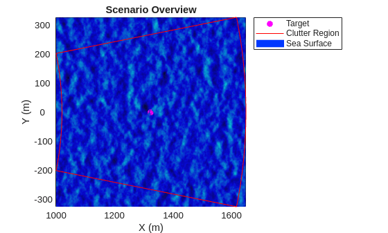
Notice that the ring-shaped clutter region covers as much of the surface as possible without going outside the surface boundary.
The advance method on the scenario is used to advance the simulation by one frame and determine if the stop time has been reached. Inside the simulation loop, start by updating the Z coordinate of the target position to match the current surface height. The receive method of the scenario is used to collect IQ signals received by radars in the scene. The return is summed over array elements and stored in the matrix PH.
frame = 0;
while advance(scenario)
    frame = frame + 1;

    % Update target position
    tgtTraj.Position(3) = height(scenario.SurfaceManager,tgtTraj.Position.') - tgtDraft;

    % Collect sum-beam range profiles
    iqsig = receive(scenario);
    PH(:,frame) = sum(iqsig{1},2);
end
Use the phased.RangeResponse object to perform matched filtering of the range profiles. The required matched filter coefficients are retrieved from the Waveform property on the radar.
resp = phased.RangeResponse(RangeMethod="Matched filter",SampleRate=Fs);
[PH,rngGates] = resp(PH,getMatchedFilter(rdr.Waveform));
Clip the data to only include range bins that contain some clutter return, as defined by the min and max radius used for the RingClutterRegion earlier.
minRng = sqrt(rdrHeight^2 + minr^2);
maxRng = sqrt(rdrHeight^2 + maxr^2);
minGate = find(rngGates >= minRng,1,'first');
maxGate = find(rngGates <= maxRng,1,'last');
rngGates = rngGates(minGate:maxGate);
PH = PH(minGate:maxGate,:);
Now plot the range-time data.
imagesc(1:numPulses,rngGates/1e3,20*log10(abs(PH)))
ch = colorbar;
ch.Title.String = 'dBW';
cl = clim;
clim([cl(2)-60, cl(2)])
set(gca,'ydir','normal')
xlabel('Pulse Index')
ylabel('Range (km)')
title('Pulse Data')
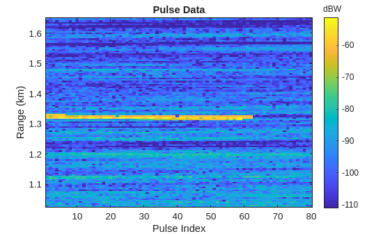
The target signal is visible around the center range, with a couple bins of range migration present.
Conclusion
In this example you simulated a stationary coastal surveillance radar with sea surface clutter. An extended cuboid target was used to emulate a ship with partial occlusion by the sea surface. Range migration of the target was visible due to the high resolution and slow update rate of the radar.