Generate Clutter and Target Returns for MTI Radar

This example shows how to generate surface clutter and target returns for the simulation of a moving target indicator (MTI) radar in a radarScenario. MTI filtering is performed and the resulting range profiles and Doppler spectra are examined. The effects of platform geometry are demonstrated by looking at both broadside and squinted trajectories, and at target placement within the radar antenna mainlobe.

rng default

MTI Radar Basics

MTI is a clutter mitigation method for pulsed radar that involves a slow-time filter and produces a time series of range profiles where returns from stationary objects have been filtered out. This is a simpler alternative to pulse-Doppler processing which does not yield a velocity estimate for targets, though direction-of-arrival estimation can still be performed on target detections.

MTI Filter

An MTI filter is a notch filter that is configured to remove the signal component at the Doppler frequency of surface clutter. Derivative filters are commonly used for their simplicity, with first- and second-order differences being the most common. This example will use the three-pulse canceller, which is a derivative filter of order 2 and length 3, and uses central differences. Such a filter is simple to implement and, since the order is 1 less than the length, it has only one null per Doppler ambiguity. In general, a balance can be found for a particular application between the width of the passband, attenuation, and the number of null frequencies.

The figure below shows the filter response for pulse cancellers of length 2 through 5 and a PRF of 5 kHz. Note that they all attenuate signals close to 0 Hz, with varying degrees of passband width and rolloff. This nominal filter type is appropriate for broadside trajectories, where clutter return is centered about 0 Hz. If using a squinted trajectory, the filter can be offset in frequency to notch out the expected frequency of the clutter centroid.

Note that spectral components of the received signals wrap at the PRF, so signals at any integer multiple of the PRF fall in the nulls of the filter. Radials speeds that impart a Doppler frequency close to these integer multiples are referred to as blind speeds because, even though the target may be in motion, its Doppler frequency is congruent to that of the clutter return. Note also that the nominal filter response is symmetric about 0 Hz, positive and negative range rates of the same magnitude are filtered similarly. The figure below shows the length-3 filter response for all Doppler frequencies between -3 and +3 multiples of the 5 kHz PRF, with the Dopplers corresponding to blind speeds indicated by vertical lines.

For a target to be detectable with range-only measurements, the target signal power must exceed that of the total clutter signal power in the target's range gate. The goal of MTI filtering is to reduce as much of the clutter signal power as possible, while preserving most of the target signal power.

Beam and Platform Geometry

Surface clutter is distributed over 360 degrees of azimuth, almost 90 degrees of elevation angle, and is bounded in range only by the horizon. When illuminated by a conical beam, the presentation of surface clutter depends on the geometry of the beam (shape and pointing direction), and on the motion of the radar platform. The detectability of a surface target with MTI processing is dependent on this clutter presentation as well as the radial speed of the target, which is defined by the absolute speed and direction of the target motion. The required positive or negative range rate for detection can depend on the location of the target within the mainlobe. A target that is located towards the high-Doppler edge of clutter might be detectable if it is moving towards the radar, but not be detectable if it is moving away from the radar at the same speed. There is thus an asymmetry in the detectable velocities for targets in all cases except for that of a broadside trajectory with the target located along the boresight vector.

The diagram below illustrates how the endoclutter region in range/cross-range changes with target speed when the target velocity is fixed in the uprange direction. In the first two subplots, the example target falls in the endoclutter region and is not detectable with MTI processing. In the 3rd subplot, the target is moving quickly enough to fall in the exoclutter region and should be detectable with MTI processing.

This next diagram illustrates how the direction of target motion affects the radial speed and thus detectability of a target. In this scenario, the target is located close to the high-Doppler edge of the beam footprint and has a constant speed of 10 m/s. Since the target is already close to the high-Doppler edge of the beam, there is a large span of directions of motion that place the target in the exoclutter region at a higher Doppler than clutter, while there is only a small span of directions of motion that place the target at a lower Doppler than clutter.

An analytical treatment is further complicated by the asymmetric beamwidth that results from any steering off broadside with a phased array, and from any rolling of the sensor frame about boresight. A physical simulation that supports such arbitrary platform geometries can be important for estimating the real-world performance of an MTI system.

Performance Metrics

While an exact solution for the detectability of a target under MTI processing is complex in general, a couple useful metrics may be computed with relative simplicity. The most commonly referenced is the minimum detectable velocity (MDV), the radial speed at which a target becomes detectable. This metric typically uses the simplifying assumption that the target lies exactly along the radar boresight. For broadside trajectories, which are the most common, this also means that the detectable velocity is symmetric about positive and negative range rates. The actual required velocity for detection is also affected by any broadening of the clutter spectrum for Doppler sidelobe control. In general, a balance must be found between broadening of the clutter spectrum and sidelobe levels required to detect the target.

Another useful metric is the MTI improvement factor, which relates the signal-to-clutter ratio (SCR) before and after MTI processing. An example demonstrating the effect of system parameters on the improvement factor is available here: MTI Improvement Factor for Land-Based Radar.

Broadside MTI Simulation

In this section, you will see how to configure a radar scenario to simulate clutter and target returns using a basic broadside trajectory. You will inspect the resulting range profiles for the case of a target that lies along the radar boresight, both above and below the MDV, then see what happens when the target is offset in the cross-range direction.

Scenario Configuration

A simulation involving radar clutter may be configured in four steps:

• Create a radar model and define system parameters and physical mounting angles

• Create a scenario container and define the Earth type, surface information, and simulation stop time

• Create scenario platforms, defining their trajectories and mounting sensors

• Create a clutter generator, defining clutter generation parameters for each radar

Configure Radar

The radarTransceiver object is used to simulate signal-level radar returns. This radar model contains sub-objects to handle various components of a monostatic radar system. Start by defining the desired system parameters, then use the provided helper function to construct the radar. Use parameters appropriate for an X-band side-looking airborne MTI radar that is configured to detect surface targets moving between about 20 to 40 mph. The antenna will be a symmetric uniform rectangular array (URA).

fc = 10e9;
prf = 7e3;
rangeRes = 20;
beamwidth = 5;
rdr = helperMakeTransceiver(beamwidth,fc,rangeRes,prf);

Set the radar mounting parameters. The radar will face out the left side of the platform (90 degree yaw), and down at the specified depression angle, with no roll about boresight.

depressionAngle = 18;
rdr.MountingAngles = [90 depressionAngle 0];

The total number of pulses collected on each activation of the radar model is defined by the NumRepetitions property. With range-only MTI processing, the pulses will be integrated noncoherently. Set the number of pulses to 64.

numPulses = 64;
rdr.NumRepetitions = numPulses;

Calculate the wavelength, Doppler and range-rate resolutions, and range gate centers for later use. The range swath extends from 0 out to the unambiguous range.

[lambda,c] = freq2wavelen(fc);
dopRes = prf/numPulses;
rangeRateRes = dop2speed(dopRes,lambda)/2;
unambRange = time2range(1/prf);
rangeGates = 0:rangeRes:(unambRange-rangeRes/2);

Configure Scenario

Create a radarScenario object. Use a flat Earth and set the update rate to 0 to indicate that the update rate should be derived from sensors in the scene.

scene = radarScenario('IsEarthCentered',false,'UpdateRate',0);

The scenario landSurface method can be used to define a homogeneous, static surface with an associated reflectivity model. Create a constant-gamma reflectivity model with the surfaceReflectivityLand function, and use a gamma value of -10 dBsm.

gamma = -10;
refl = surfaceReflectivityLand('Model','ConstantGamma','Gamma',gamma);
landSurface(scene,'RadarReflectivity',refl);

Configure Platforms

Create the radar platform. Let the platform fly a straight-line trajectory at the specified altitude and speed. The platform will move in the +X direction at 180 m/s.

altitude = 2e3;
rdrspd = 180;
rdrtraj = kinematicTrajectory('Position',[0 0 altitude],'Velocity',[rdrspd 0 0]);
rdrplat = platform(scene,'Sensors',rdr,'Trajectory',rdrtraj);

Create a target platform that lies on the surface along the antenna boresight, and give it a velocity vector such that the return signal will be separated from clutter in Doppler. Start by calculating the expected spread of clutter in Doppler. For broadside geometries and a symmetric beam, the two-sided extent of clutter in Doppler, ${\mathit{W}}_{\mathit{D}}$, can be calculated with a simple equation:

$${\mathit{W}}_{\mathit{D}}=\frac{4}{\lambda }|\mathit{v}|\sin \left(\frac{\theta }{2}\right)$$

where $\lambda$ is the wavelength, $|\mathit{v}|$ is the radar speed, and $\theta$is the two-sided beamwidth. In reality, Doppler sidelobes will extend beyond this width, and this width may be increased by slow-time windowing. The MDV may be seen as a function of this width and of the MTI filter response. Calculate the Doppler width of clutter.

Wd = 4/lambda*rdrspd*sind(beamwidth/2);

To place the target along the antenna boresight, calculate the required ground range from the radar altitude and boresight depression angle. Recall that the radar is pointed in the +Y direction.

gndrng = altitude/tand(depressionAngle);
tgtrng = sqrt(gndrng^2 + altitude^2);
bspos = [0 gndrng 0];

Calculate a closing rate that places the target at 500 Hz greater than the high-Doppler clutter edge. Use the helper function to calculate the required speed for a target moving in the -Y direction, and create a kinematic trajectory.

tgtClosingRate = (Wd/2 + 500)*lambda/2;
tgtvel = helperTargetVelocityFromClosing(rdrplat.Position,rdrplat.Trajectory.Velocity,bspos,tgtClosingRate);
tgttraj = kinematicTrajectory('Position',bspos,'Velocity',tgtvel);

In order to understand the effect of the MTI filter on detectability, express the target RCS in terms of the expected clutter RCS. The NRCS can be found using the reflectivity model created earlier, and clutterSurfaceRCS can be used to approximate the total RCS of clutter in the range gate containing the target and within the span of the mainlobe. Express the RCS in dBsm.

clutterNRCS = refl(depressionAngle,fc);
clutterRCS = clutterSurfaceRCS(clutterNRCS,tgtrng,beamwidth,beamwidth,depressionAngle,rdr.Waveform.PulseWidth,c);
clutterRCS = 10*log10(clutterRCS);

Set the target RCS to be 8 dBsm less than the clutter RCS. Without any processing, the target will not be detectable.

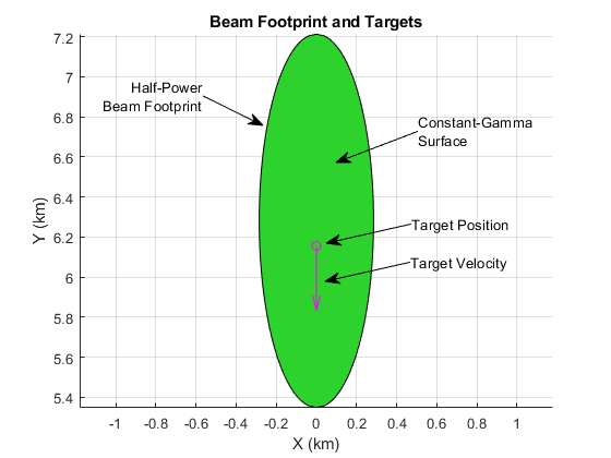
tgtrcs = clutterRCS - 8; % dBsm
tgtplat = platform(scene,'Trajectory',tgttraj,'Signatures',rcsSignature('Pattern',tgtrcs));

The figure below shows the beam footprint with this scenario, and the location and velocity vector of the target.

Configure Clutter Generation

Finally, create a ClutterGenerator and specify clutter generation settings. Set the clutter resolution to one half of the radar range resolution to ensure multiple clutter patches per resolution cell (the range resolution is smaller than the cross-range resolution with this radar configuration). Set UseBeam to true to generate mainlobe clutter.

clutterGenerator(scene,rdr,'Resolution',rangeRes/2,'UseBeam',true);

Simulate Clutter and Target Return Signals

Use the scenario receive method to collect one interval of pulse data. The result is formatted as fast time-by-slow time, and is referred to as a phase history (PH) matrix. This sum beam is an accumulation of the typical radar data cube across channels. The output will be a cell array, with one cell for each radarTransceiver in the scene. This scenario has only one radar, so unpack PH into a matrix by accessing the first element.

PH = receive(scene);
PH = PH{1};

Process the PH data with the MTI filter using the provided helper function. The resulting matrix will be formatted similarly to the original PH matrix, except it has been filtered along the slow-time dimension and has 2 fewer pulses of data to omit the invalid initial filter outputs. The filter has been normalized by the expected noise gain for easier comparison of the results.

PH_mti = helperMTIFilter(PH);

Plot the original phase history matrix alongside the filtered matrix.

helperPlotPhaseHistory(PH,PH_mti,rangeGates)

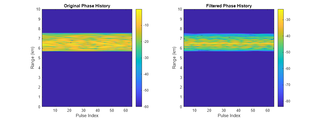
In the filtered phase history, the target return is visible above clutter on most pulses.

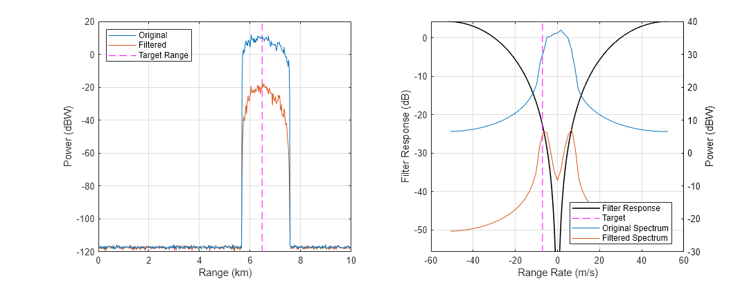
To average out the small fluctuations in clutter and target power, MTI systems will often perform a noncoherent integration of the filtered pulses to form a final range profile. Use the pulsint function to form range profiles from the original PH matrix and the filtered PH matrix. Use the provided helper function to plot the range profiles along with the filter response and annotations indicating the target range and radial speed. The Doppler spectra before and after filtering are also shown. These spectra are computed by accumulating the power in each Doppler bin over all range gates.

rangeProfile = pulsint(PH);
rangeProfile_mti = pulsint(PH_mti);
helperPlotMTI(rdrplat,tgtplat,rangeProfile,rangeProfile_mti,rangeGates,prf,lambda,PH,PH_mti)

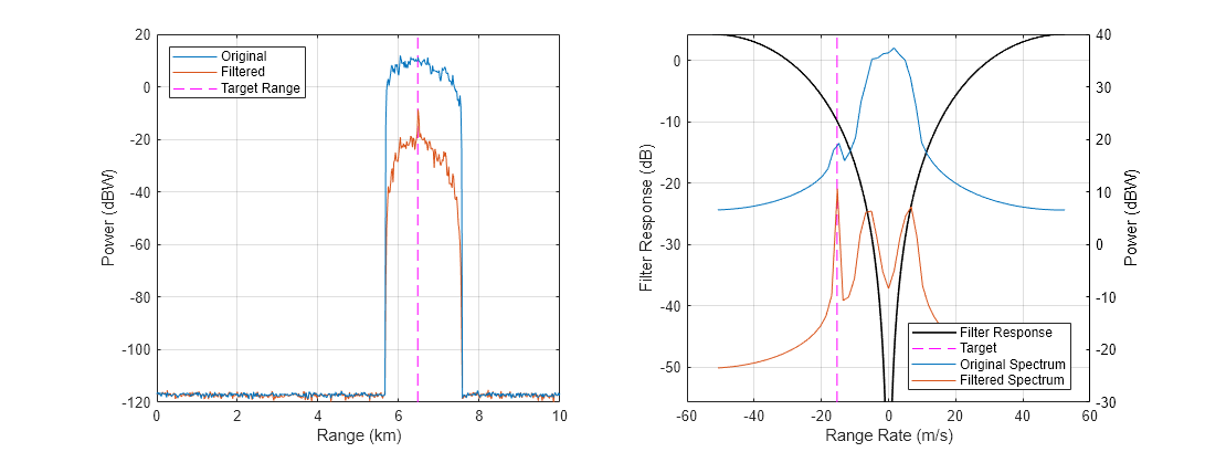
In the original range profile, the target return is not detectable over clutter. In the filtered range profile, a peak at the target range is clearly visible.

The target was separated from the edge of clutter by 500 Hz. The signal component at the Doppler frequency of the target saw an attenuation by about 10 dB while clutter was attenuated by about 21 dB at the high-Doppler edge, which is the minimum attenuation seen by the mainlobe clutter signal (not including Doppler sidelobes). After filtering, the total clutter power in a range bin is dominated by the least-attenuated component of the signal, so the total gain in SCR is at least 21-10=11 dB. Since the clutter RCS was only 8 dBsm greater than the target RCS, this gain in SCR is sufficient to detect the target.

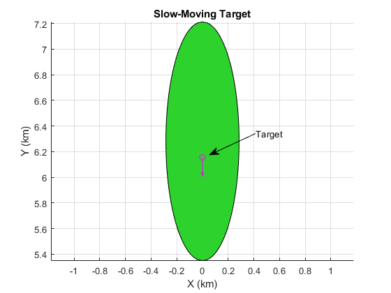
Now adjust the target velocity to place it 50 Hz lower than the high-Doppler edge of the clutter return.

tgtClosingRate = (Wd/2 - 50)*lambda/2;
tgtvel = helperTargetVelocityFromClosing(rdrplat.Position,rdrplat.Trajectory.Velocity,bspos,tgtClosingRate);
tgttraj.Velocity = tgtvel;

The figure below shows the beam footprint with this slow-moving target.

Use the provided helper function to re-run the scenario and collect results.

[rangeProfile,rangeProfile_mti,PH,PH_mti] = helperRunMTIScenario(scene);

Plot the resulting range profiles, filter response, and spectra.

helperPlotMTI(rdrplat,tgtplat,rangeProfile,rangeProfile_mti,rangeGates,prf,lambda,PH,PH_mti)

In this case, the target signal is not benefitting from any gain over the clutter signal, and is not detectable.

Offset Target Position

Now, without changing the velocity vector, offset the target from the boresight-ground intersection point by 260 m in the +X direction. Because this is the direction of radar motion, the target is now close to the high-Doppler edge of the clutter signal.

tgttraj.Position = bspos + [260 0 0];

The figure below shows this new geometry.

Repeat the simulation and plot the results.

[rangeProfile,rangeProfile_mti,PH,PH_mti] = helperRunMTIScenario(scene);
helperPlotMTI(rdrplat,tgtplat,rangeProfile,rangeProfile_mti,rangeGates,prf,lambda,PH,PH_mti)

While not as prominent as in the case of the fast-moving target, a peak corresponding to the target range can be seen thanks to the off-broadside location of the target within the mainlobe.

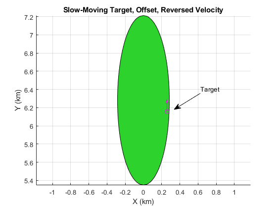
Now, with the target still offset towards the high-Doppler edge of the clutter signal, reverse the direction of the target velocity vector.

tgttraj.Velocity = -tgttraj.Velocity;

[rangeProfile,rangeProfile_mti,PH,PH_mti] = helperRunMTIScenario(scene);
helperPlotMTI(rdrplat,tgtplat,rangeProfile,rangeProfile_mti,rangeGates,prf,lambda,PH,PH_mti)

The peak has again disappeared thanks to the opposing influence of the target position within the mainlobe and its velocity vector.

Squinted MTI Simulation

In this section you will simulate MTI filtering of squinted beam data in order to inspect the asymmetry in the detectable velocities across range. Mainlobe clutter under a squinted beam will exhibit slant: a varying Doppler centroid over range. If a single MTI filter is used across all range gates, this means that the effectiveness of the filter could vary over range.

The radar MountingAngles property can be used to rotate the radar frame so that the boresight is pointed as desired. The depression angle will be kept constant. Use a forward-squinted trajectory. Release the radar and set the mounting angles.

azPointing = 10;
release(rdr)
rdr.MountingAngles = [azPointing depressionAngle 0];

Get the antenna boresight direction, and a ground-projected boresight vector for placing targets on the ground along the same direction.

[bs(1),bs(2),bs(3)] = sph2cart(azPointing*pi/180,-depressionAngle*pi/180,1);
bsxy = [bs(1:2)/norm(bs(1:2)) 0];

Calculate approximate range and Doppler clutter centroids from the boresight vector. This will be used to place targets at ranges and Dopplers relative to clutter.

centerRange = -altitude/bs(3);
centerDop = 2/lambda*rdrspd*cosd(azPointing)*cosd(depressionAngle);

Select a closing rate that puts the targets 200 Hz above the calculated clutter centroid.

tgtClosingRate = (centerDop + 200)*lambda/2

tgtClosingRate = 171.5873

Place the first target platform along the boresight vector (as in the last section), calculate the required velocity vector, and update the trajectory properties.

tgtrng1 = centerRange;
tgtpos1 = sqrt(tgtrng1^2-altitude^2)*bsxy;
tgtvel1 = helperTargetVelocityFromClosing(rdrplat.Position,rdrplat.Trajectory.Velocity,tgtpos1,tgtClosingRate);
tgttraj.Position = tgtpos1;
tgttraj.Velocity = tgtvel1;

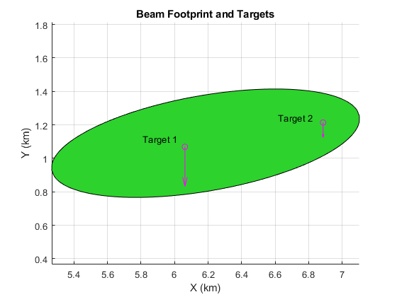
Create a second platform and place it 800 m further along the boresight direction, and give it the same closing rate.

tgtrng2 = centerRange + 800;
tgtpos2 = sqrt(tgtrng2^2-altitude^2)*bsxy;
tgtvel2 = helperTargetVelocityFromClosing(rdrplat.Position,rdrplat.Trajectory.Velocity,tgtpos2,tgtClosingRate);
tgttraj2 = kinematicTrajectory('Position',tgtpos2,'Velocity',tgtvel2);
tgtplat(2) = platform(scene,'Trajectory',tgttraj2,'Signatures',rcsSignature('Pattern',tgtrcs));

The figure below shows the location of the beam footprint, targets, and their velocity vectors.

Run the simulation and plot the resulting range profiles, filter response, and spectra.

[rangeProfile,rangeProfile_mti,PH,PH_mti] = helperRunMTIScenario(scene,true,centerDop/prf);
helperPlotMTI(rdrplat,tgtplat,rangeProfile,rangeProfile_mti,rangeGates,prf,lambda,PH,PH_mti,centerDop)

The first important observation of the range profiles is the inflection point around the center range. The low- and high-range sides of the clutter return were offset from the Doppler centroid by a larger amount than in the broadside case, and experienced lower attenuation than the attenuation at the centroid. As such, the target signal at that range is visible in the filtered data. The second target at a greater range is not visible because the clutter return at that range was not attenuated as well.

Note that in this scenario, while the platforms are moving at speeds of about 18 and 7 m/s for targets 1 and 2 respectively, their closing rates are both large enough (about 172 m/s) to be ambiguous and appear as if they are moving away from the radar at about 40 m/s. This range-rate ambiguity would typically be resolved by using multiple PRFs or by feeding measurements into a tracker.

To better see the range dependence on the clutter Doppler spectra, plot the full range-Doppler map (RDM) before and after filtering, using the provided helper function. The displayed region will be between 4 and 9 km range and -3.5 to -2 kHz to see the data more clearly.

helperPlotRDM(PH,PH_mti,rangeGates,prf,lambda,rdrplat,tgtplat)

From the RDM it can be seen that much of the clutter signal at the range of the first target (about 6.5 km) has been attenuated below the target signal power, while the clutter signal at the range of the second target has not been as well attenuated.

Conclusion

In this example you saw how to configure a radar scenario to generate target and clutter returns appropriate for simulation of MTI performance. The effect of target placement and direction of motion with the mainlobe during both broadside and squinted collections was demonstrated.

Supporting Functions

helperMakeTransceiver

function [rdr,bw] = helperMakeTransceiver( bw,fc,rangeRes,prf )
% This helper function creates a radarTransceiver from some basic system
% parameters.

c = physconst('lightspeed');

rdr = radarTransceiver;

rdr.TransmitAntenna.OperatingFrequency = fc;
rdr.ReceiveAntenna.OperatingFrequency = fc;

sampleRate = c/(2*rangeRes);
sampleRate = prf*round(sampleRate/prf); % adjust to match constraint with PRF

rdr.Receiver.SampleRate = sampleRate;
rdr.Waveform.SampleRate = sampleRate;
rdr.Waveform.PulseWidth = 2*rangeRes/c;
rdr.Waveform.PRF = prf;

% Create a rectangular array with a beamwidth close to the specification
N = round(0.8859*2./(bw(:).'*pi/180));
bw = 0.8859*2./N*180/pi; % Achieved beamwidth
N = flip(N);
lambda = freq2wavelen(fc,c);
array = phased.URA(N,lambda/2);
az = -180:.4:180;
el = -90:.4:90;
G = pattern(array,fc,az,el,'Type','efield','normalize',false);
M = 20*log10(abs(G));
P = angle(G);
E = phased.CustomAntennaElement('FrequencyVector',[fc-1 fc+1],...
    'AzimuthAngles',az,'ElevationAngles',el,'MagnitudePattern',M,'PhasePattern',P);
rdr.TransmitAntenna.Sensor = E;
rdr.ReceiveAntenna.Sensor = E;

end

helperTargetVelocityFromClosing

function vel = helperTargetVelocityFromClosing( rdrpos,rdrvel,tgtpos,tgtClosingRate )
% Calculates the required speed in the -Y direction for the target platform
% to have the desired closing rate.

los = rdrpos(:) - tgtpos(:);
los = los/norm(los);
spd = (tgtClosingRate + dot(rdrvel(:),los))/los(2);
vel = [0 spd 0];

end

helperMTIFilter

function y = helperMTIFilter( x,cdn )
% Filter the input x across the second dimension using a second-order
% central difference.

% Filter coefficients
h = [1 -2 1];

% If non-zero center Doppler, apply phase ramp to filter coefficients
if nargin > 1
   phi = 2*pi*cdn*(0:numel(h)-1);
   h = h.*exp(1i*phi);
end

% Run filter and omit invalid output samples
y = filter(h,1,x,[],2);
y = y(:,numel(h):end);

% Normalize by the noise gain
y = y/sqrt(sum(abs(h).^2));

end

helperPlotPhaseHistory

function helperPlotPhaseHistory( PH,PH_mti,rg )
% This function plots the phase history matrices from before and after MTI
% filtering

figure;
set(gcf,'Position',get(gcf,'Position')+[0 0 560 0])

% Limit displayed ranges to 10 km
maxRange = 10e3;
maxGate = find(rg <= maxRange,1,'last');
rg = rg(1:maxGate);
PH = PH(1:maxGate,:);
PH_mti = PH_mti(1:maxGate,:);

numPulses = size(PH,2);

subplot(1,2,1)
imagesc(1:numPulses,rg/1e3,20*log10(abs(PH)))
set(gca,'ydir','normal')
cx = clim;
clim([cx(2)-60 cx(2)])
colorbar
xlabel('Pulse Index')
ylabel('Range (km)')
title('Original Phase History')

subplot(1,2,2)
imagesc(3:numPulses,rg/1e3,20*log10(abs(PH_mti)))
set(gca,'ydir','normal')
cx = clim;
clim([cx(2)-60 cx(2)])
colorbar
xlabel('Pulse Index')
ylabel('Range (km)')
title('Filtered Phase History')

end

helperPlotMTI

function helperPlotMTI( rdrplat,tgtplat,rp,rp_mti,rg,prf,lambda,PH,PH_mti,centerDop )
% This function plots the range profiles from before and after MTI
% processing, and plots the filter response along with the clutter spectrum
% and annotations.

fh = figure;

% Calculate range/Doppler to tgt
for ind = 1:numel(tgtplat)
    tgtrng(ind) = norm(rdrplat.Position - tgtplat(ind).Position);
    los = (rdrplat.Position-tgtplat(ind).Position)/tgtrng(ind);
    tgtClosingRate(ind) = sum((tgtplat(ind).Trajectory.Velocity-rdrplat.Trajectory.Velocity).*los);
    tgtdop(ind) = 2/lambda*tgtClosingRate(ind);
end

% Limit displayed ranges to 10 km
maxRange = 10e3;
maxGate = find(rg <= maxRange,1,'last');
rg = rg(1:maxGate);
rp = rp(1:maxGate);
rp_mti = rp_mti(1:maxGate);

% Range-power plots
subplot(1,2,1)

% Plot range profiles
hndls1(1) = plot(rg/1e3,20*log10(rp)); % original
hold on
hndls1(2) = plot(rg/1e3,20*log10(rp_mti)); % filtered

% Plot truth target ranges
for ind = 1:numel(tgtrng)
   hndls1(3) = line([1 1]*tgtrng(ind)/1e3,ylim,'color','magenta','linestyle','--');
end
hold off
grid on
xlabel('Range (km)')
ylabel('Power (dBW)')
set(gca,'Children',flip(get(gca,'Children')))
legend(hndls1,{'Original','Filtered','Target Range'},'Location','NorthWest')

% Spectrum plots
subplot(1,2,2)

% Plot filter response
h = [1 -2 1];
if nargin > 9
    phi = 2*pi*centerDop/prf*(0:numel(h)-1);
    h = h.*exp(1i*phi);
end
f = linspace(-prf/2,prf/2,1e3);
rr = -lambda/2*f;
hresp = freqz(h,1,f,prf);
hresp = hresp/sqrt(sum(h.^2)); % normalize to keep noise floor constant
hresp = 20*log10(abs(hresp));
hndls2(1) = plot(rr,hresp,'black','linewidth',1.2);
mn = max(max(hresp)-60,min(hresp)); % limit to 60 dB down
ylim([mn max(hresp)])
hold on

% Plot annotation at tgt RR
tgtdop = mod(tgtdop+prf/2,prf)-prf/2;
tgtrr = -tgtdop*lambda/2;
for ind = 1:numel(tgtrr)
    hndls2(2) = line([1 1]*tgtrr(ind),ylim,'color','magenta','linestyle','--');
end

xlabel('Range Rate (m/s)')
ylabel('Filter Response (dB)')

% Get before/after Doppler spectra and plot
numPulses = size(PH,2);
rrBins = -(-prf/2:prf/numPulses:(prf/2-prf/numPulses))*lambda/2;
RDM = fftshift(fft(PH,[],2),2);
dopSpec = sum(abs(RDM).^2,1);
numPulses_mti = size(PH_mti,2);
rrBins_mti = -(-prf/2:prf/numPulses_mti:(prf/2-prf/numPulses_mti))*lambda/2;
RDM_mti = fftshift(fft(PH_mti,[],2),2);
dopSpec_mti = sum(abs(RDM_mti).^2,1);

yyaxis right
hndls2(3) = plot(rrBins,10*log10(abs(dopSpec)),'Color',hndls1(1).Color,'linestyle','-');
hndls2(4) = plot(rrBins_mti,10*log10(abs(dopSpec_mti)),'Color',hndls1(2).Color,'linestyle','-');
hold off
grid on
ylabel('Power (dBW)')
set(gca,'YColor','black')

legend(hndls2,{'Filter Response','Target','Original Spectrum','Filtered Spectrum'},'Location','Best')

set(fh,'Position',get(fh,'Position')+[0 0 560 0])

end

helperRunMTIScenario

function [ rp,rp_mti,PH,PH_mti,RDM ] = helperRunMTIScenario( scene,doRestart,centerDopNorm )

if nargin < 2
    doRestart = true;
end

if nargin < 3
    centerDopNorm = 0;
end

if doRestart
    restart(scene)
end

% Call scenario receive method
PH = receive(scene);
PH = PH{1};

% Perform MTI filtering
PH_mti = helperMTIFilter(PH,centerDopNorm);

% Generate before/after range profiles
rp = pulsint(PH);
rp_mti = pulsint(PH_mti);

% Perform Doppler processing
RDM = fftshift(fft(PH,[],2),2);

end

helperPlotRDM

function helperPlotRDM( PH,PH_mti,rg,prf,lambda,rdrplat,tgtplat )

figure;
set(gcf,'Position',get(gcf,'Position')+[0 0 560 0])

% Calculate range/Doppler to tgt
for ind = 1:numel(tgtplat)
    tgtrng(ind) = norm(rdrplat.Position - tgtplat(ind).Position);
    los = (rdrplat.Position-tgtplat(ind).Position)/tgtrng(ind);
    tgtClosingRate(ind) = sum((tgtplat(ind).Trajectory.Velocity-rdrplat.Trajectory.Velocity).*los);
    tgtdop(ind) = 2/lambda*tgtClosingRate(ind);
end
tgtdop = mod(tgtdop+prf/2,prf)-prf/2;

% Limit displayed ranges to 3-10 km
maxRange = 9e3;
minRange = 4e3;
maxGate = find(rg <= maxRange,1,'last');
minGate = find(rg >= minRange,1,'first');
rg = rg(minGate:maxGate);
PH = PH(minGate:maxGate,:);
PH_mti = PH_mti(minGate:maxGate,:);

maxDop = -2e3;

subplot(1,2,1)
RDM = fftshift(fft(PH,[],2),2);
numPulses = size(PH,2);
dopBins = -prf/2:prf/numPulses:prf/2-prf/numPulses;
maxDopBin = find(dopBins <= maxDop,1,'last');
imagesc(dopBins(1:maxDopBin),rg/1e3,20*log10(abs(RDM(:,1:maxDopBin))))
for ind = 1:numel(tgtplat)
    line(xlim,[1 1]*tgtrng(ind)/1e3,'color','magenta','linestyle','--')
    line([1 1]*tgtdop(ind),ylim,'color','magenta','linestyle','--')
end
set(gca,'ydir','normal')
cx = clim;
clim([cx(2)-60 cx(2)])
colorbar
xlabel('Doppler (Hz)')
ylabel('Range (km)')
title('Original RDM')

subplot(1,2,2)
RDM_mti = fftshift(fft(PH_mti,[],2),2);
numPulses_mti = size(PH_mti,2);
dopBins_mti = -prf/2:prf/numPulses_mti:prf/2-prf/numPulses_mti;
maxDopBin = find(dopBins_mti <= maxDop,1,'last');
imagesc(dopBins_mti(1:maxDopBin),rg/1e3,20*log10(abs(RDM_mti(:,1:maxDopBin))))
for ind = 1:numel(tgtplat)
    line(xlim,[1 1]*tgtrng(ind)/1e3,'color','magenta','linestyle','--')
    line([1 1]*tgtdop(ind),ylim,'color','magenta','linestyle','--')
end
set(gca,'ydir','normal')
cx = clim;
clim([cx(2)-60 cx(2)])
colorbar
xlabel('Doppler (Hz)')
ylabel('Range (km)')
title('Filtered RDM')

end