Barrage Jammer
Support for Modeling Barrage Jammer
The barrageJammer object models a broadband jammer. The output of barrageJammer is a complex white Gaussian noise sequence. The modifiable properties of the barrage jammer are:
ERP— Effective radiated power in wattsSamplesPerFrameSource— Source of number of samples per frameSamplesPerFrame— Number of samples per frameSeedSource— Source of seed for random number generatorSeed— Seed for random number generator
The real and imaginary parts of the complex white Gaussian noise sequence each have variance equal to 1/2 the effective radiated power in watts. Denote the effective radiated power in watts by P. The barrage jammer output is:
In this equation, x[n] and y[n] are uncorrelated sequences of zero-mean Gaussian random variables with unit variance.
Model Barrage Jammer Output
This example examines the statistical properties of the barrage jammer output and how they relate to the effective radiated power (ERP). Create a barrage jammer using an effective radiated power of 5000 watts. Generate output at 500 samples per frame. Then call the step function once to generate a single frame of complex data. Using the histogram function, show the distribution of barrage jammer output values. The BarrageJammer System object™ uses a random number generator. In this example, the random number generator seed is fixed for illustrative purposes and can be removed.
rng default
jammer = barrageJammer('ERP',5000,...
    'SamplesPerFrame',500);
y = jammer();
subplot(2,1,1)
histogram(real(y))
title('Histogram of Real Part')
subplot(2,1,2)
histogram(imag(y))
title('Histogram of Imaginary Part')
xlabel('Watts')
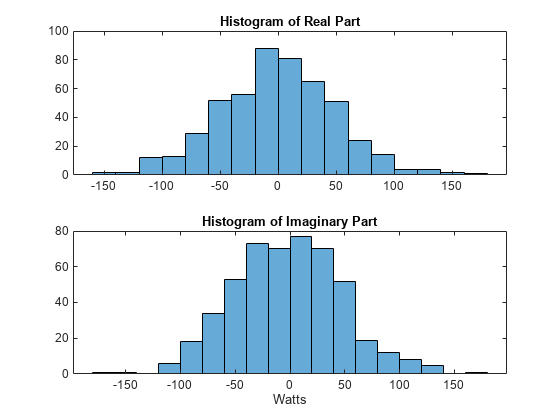
The mean values of the real and imaginary parts are
mean(real(y))
ans =
-1.0961
mean(imag(y))
ans =
-2.1671
which are effectively zero. The standard deviations of the real and imaginary parts are
std(real(y))
ans =
50.1950
std(imag(y))
ans =
49.7448
which agree with the predicted value of .
Model Effect of Barrage Jammer on Target Echo
This example demonstrates how to simulate the effect of a barrage jammer on a target echo. First, create the required objects. You need an array, a transmitter, a radiator, a target, a jammer, a collector, and a receiver. Additionally, you need to define two propagation paths: one from the array to the target and back, and the other path from the jammer to the array.
antenna = phased.ULA(4);
Fs = 1e6;
fc = 1e9;
rng('default')
waveform = phased.RectangularWaveform('PulseWidth',100e-6,...
    'PRF',1e3,'NumPulses',5,'SampleRate',Fs);
transmitter = phased.Transmitter('PeakPower',1e4,'Gain',20,...
    'InUseOutputPort',true);
radiator = phased.Radiator('Sensor',antenna,'OperatingFrequency',fc);
jammer = barrageJammer('ERP',1000,...
    'SamplesPerFrame',waveform.NumPulses*waveform.SampleRate/waveform.PRF);
target = phased.RadarTarget('Model','Nonfluctuating',...
    'MeanRCS',1,'OperatingFrequency',fc);
targetchannel = phased.FreeSpace('TwoWayPropagation',true,...
    'SampleRate',Fs,'OperatingFrequency', fc);
jammerchannel = phased.FreeSpace('TwoWayPropagation',false,...
    'SampleRate',Fs,'OperatingFrequency', fc);
collector = phased.Collector('Sensor',antenna,...
    'OperatingFrequency',fc);
amplifier = phased.ReceiverPreamp('EnableInputPort',true);
Assume that the array, target, and jammer are stationary. The array is located at the global origin, (0,0,0). The target is located at (1000,500,0), and the jammer is located at (2000,2000,100). Determine the directions from the array to the target and jammer.
targetloc = [1000 ; 500; 0];
jammerloc = [2000; 2000; 100];
[~,tgtang] = rangeangle(targetloc);
[~,jamang] = rangeangle(jammerloc);
Finally, transmit the rectangular pulse waveform to the target, reflect it off the target, and collect the echo at the array. Simultaneously, the jammer transmits a jamming signal toward the array. The jamming signal and echo are mixed at the receiver. Generate waveform.
wav = waveform();
% Transmit waveform
[wav,txstatus] = transmitter(wav);
% Radiate pulse toward the target
wav = radiator(wav,tgtang);
% Propagate pulse toward the target
wav = targetchannel(wav,[0;0;0],targetloc,[0;0;0],[0;0;0]);
% Reflect it off the target
wav = target(wav);
% Collect the echo
wav = collector(wav,tgtang);
Generate the jamming signal.
jamsig = jammer();
% Propagate the jamming signal to the array
jamsig = jammerchannel(jamsig,jammerloc,[0;0;0],[0;0;0],[0;0;0]);
% Collect the jamming signal
jamsig = collector(jamsig,jamang);

% Receive target echo alone and target echo + jamming signal
pulsewave = amplifier(wav,~txstatus);
pulsewave_jamsig = amplifier(wav + jamsig,~txstatus);
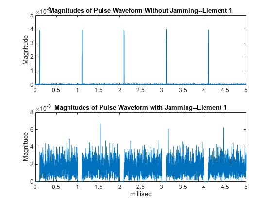
Plot the result, and compare it with received waveform with and without jamming.
subplot(2,1,1)
t = unigrid(0,1/Fs,size(pulsewave,1)*1/Fs,'[)');
plot(t*1000,abs(pulsewave(:,1)))
title('Magnitudes of Pulse Waveform Without Jamming--Element 1')
ylabel('Magnitude')
subplot(2,1,2)
plot(t*1000,abs(pulsewave_jamsig(:,1)))
title('Magnitudes of Pulse Waveform with Jamming--Element 1')
xlabel('millisec')
ylabel('Magnitude')