seareflectivity

Normalized sea surface reflectivity

Since R2021a

Syntax

nrcs = seareflectivity(scale,graz,freq)

nrcs = seareflectivity(___,Polarization = pol)

nrcs = seareflectivity(___,ScaleType = scaletype)

nrcs = seareflectivity(___,Model = model)

nrcs = seareflectivity(___,LookAngle = lookang)

[nrcs,hgtsd,beta0,windvelocity] = seareflectivity(___)

Description

nrcs = seareflectivity(scale,graz,freq) returns the normalized sea surface reflectivity nrcs for the sea state scale at the grazing angle graz with the transmitted frequency freq. In this syntax, sea surface reflectivity is calculated using the NRL Sea Clutter Model by Gregers-Hansen and Mittal. The reflectivity is also called the normalized radar cross section (NRCS) and denoted σ⁰.

nrcs = seareflectivity(___,Polarization = pol) also specifies the polarization pol of the transmitted wave. Polarization can be horizontal or vertical.

nrcs = seareflectivity(___,ScaleType = scaletype) also specifies the scale type scaletype which is either sea state 'SeaState' or wind scale 'WindScale'.

nrcs = seareflectivity(___,Model = model) also specifies the reflectivity model.

nrcs = seareflectivity(___,LookAngle = lookang) also specifies the look angle lookang, which is compatible with select model types.

[nrcs,hgtsd,beta0,windvelocity] = seareflectivity(___) returns additional outputs:

• hgtsd — Standard deviation of the surface height for the specified sea state number.

• beta0 — Slope of the sea type. beta0 is 1.4 times the root mean square (RMS) surface slope. The surface σ⁰ value for sea clutter reflectivity is computed based on the NRL Sea Clutter Model by Gregers-Hansen and Mittal.

• windvelocity — Wind velocity.

Examples

NRCS of Sea Clutter Patch

Calculate the NRCS of a sea clutter patch. Assume that the patch is the sea with sea state number equal to 2 and the radar system operates at a frequency of 30 GHz. Also assume the grazing angle is 10 degrees.

scale = 2;    
graz = 10;  
freq = 30e9;

Calculate the normalized NRCS for the sea clutter patch.

nrcs = seareflectivity(scale,graz,freq)

nrcs = 
2.1555e-04

You can use the normalized RCS to calculate the total clutter patch RCS.

Polarized Sea Reflectivity

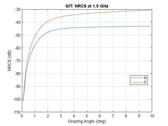
Calculate and plot the horizontal and vertical reflectivities from the GIT model. The radar operates at an L-band frequency of 1.5 GHz at grazing angles from 0.1 to 10 degrees. Assume sea state 3.

seastate = 3;
graz = 0.1:0.2:10;
freq = 1.5e9;
model = 'GIT';

Compute the horizontal and vertical polarized reflectivities.

reflh = seareflectivity(seastate,graz,freq, ...
    Model = model,Polarization = 'H');
reflv = seareflectivity(seastate,graz,freq, ...
    Model = model,Polarization = 'V');

Plot the reflectivities as a function of grazing angle.

plot(graz,pow2db(reflh))
hold on
grid on
plot(graz,pow2db(reflv))
legend('H','V','Location','Best')
xlabel('Grazing Angle (deg)')
ylabel('NRCS (dB)')
title('GIT: NRCS at 1.5 GHz')

Input Arguments

scale — Sea state or wind scale

nonnegative integer

If you set scaletype to 'SeaState', scale is interpreted as the sea state, specified as a nonnegative scalar between [0,8]. If you set scaletype to 'WindScale', scale is interpreted as the Beaufort wind scale, specified as a positive scalar between [1,9].

Dependency

The interpretation of the scale argument depends on the value of scaletype name-value pair.

graz — Grazing angle

nonnegative scalar | N-length vector of grazing values

Grazing angle, specified as a nonnegative scalar or an N-length row vector of nonnegative values. This argument specifies the grazing angles of the clutter patch relative to the radar. Units are in degrees. See grazingang.

freq — Transmitted frequencies

R-length vector of positive values

Transmitted frequencies, specified as a positive scalar or R-length vector of positive values. Units are in Hz.

Example: freq = 70e9

pol — Polarization of transmitted wave

'H' (default) | 'V'

Polarization of transmitted wave, specified as 'H' for horizontal polarization or 'V' for vertical polarization.

Example: 'V'

scaletype — Scale type

'SeaState' (default) | 'WindScale'

Scale type, specified as either:

• 'SeaState' — The function uses the Sea State model. When you specify this option, the scale input scale must be a nonnegative scalar between [0,8].

• 'WindScale' — The function uses the Beaufort Wind Scale model. When you specify this option, the scale input scale must be a positive scalars between [1,9].

Example: 'WindScale'

model — Sea reflectivity model

'NRL' (default) | 'APL' | 'GIT' | 'Hybrid' | 'Masuko' | 'Nathanson' | 'RRE' | 'Sittrop' | 'TSC'

Sea reflectivity model, specified as 'NRL', 'APL', 'GIT', 'Hybrid', 'Masuko', 'Nathanson', 'RRE', 'Sittrop', or 'TSC'. The table Sea Reflectivity Models summarizes the sea surface models available in the radar simulation and their domains of application.

lookang — Radar look angle

0 (default) | nonnegative scalar | 'Upwind' | 'Downwind' | 'Crosswind'

Radar look angle, specified as a nonnegative scalar between 0° and 180° or as:

• 'Upwind' – 0°

• 'Downwind' – 180°

• 'Crosswind' – 90°

Radar look angle is zero when looking upwind.

Dependencies

To enable this argument, set the model name to 'APL', 'GIT', 'Hybrid', 'Masuko', 'Sittrop', or 'TSC'.

Data Types: double

Output Arguments

nrcs — Normalized surface reflectivity

real-valued N-by-R matrix

Normalized surface reflectivity, returned as a real-valued N-by-R matrix. N is the length of the grazing angle graz or, for land surfaces only, depression angle. R is the length of the frequency vector freq. nrcs is dimensionless but often expressed as m²/m². Normalized reflectivity is also called normalized radar cross section (NRCS).

hgtsd — Standard deviation of surface height

scalar

Standard deviation of the surface height, returned as a scalar. The model for height deviation, surface slope, and wind velocity is based on a model by Barton. Units are in meters.

beta0 — Slope of the sea type

scalar

Slope of the sea type β₀, returned as a scalar. The model for height deviation, surface slope, and wind velocity is based on a model by Barton. Units are in degrees.

windvelocity — Wind velocity

scalar

Wind velocity, returned as a scalar. The model for the height deviation, surface slope, and wind velocity is based on a model by Barton. Units are in meters per second.

More About

Sea Reflectivity Models

Model	Type	Grazing Angles	Frequency Range	Sea State
'NRL' – Sea Clutter Model due to Gregers-Hansen and Mittal. (Default model) Naval Research Laboratory empirical model for sea reflectivity. The model does not include variation with azimuth or wind direction. The model matches experimental results with an absolute deviation of about 2.2 to 2.3 dB for grazing angles from 0.1° to 10°. A deviation of 2.6 dB can be seen for grazing angles above 10° and below 60°. See [1] and [2].	Empirical model	0.1° – 60°	0.5 – 35 GHz	0 – 6
'APL' – John Hopkins Applied Physics Laboratory ADSAM model. Derived wind velocity from sea state produces less conservative reflectivity values than GIT model at lower sea states. Takes into account wave height and wave speed. Differs from the GIT model by deriving wind velocity from sea state. See [3].	Semi-empirical	0.1 – 10	1 – 100	1 – 6
'GIT' – Georgia Institute of Technology Semi-empirical model based on multipath, wind speed, and wind direction factor. Takes into account wave height and wave speed. Derived wind velocity from sea state produces less conservative reflectivity values than GIT at lower sea states. [5] and [1].	Semi-empirical	0.1 – 10	1 – 100	1 – 6
'Hybrid' – Hybrid model that mixes work by Barton, Nathanson's tables, and GIT semi-empirical models. May be biased high in the low grazing angle regime. See [5].	Semi-empirical	0.1 – 30	0.5 – 35	0 – 5
'Masuko' -- Empirical model applicable for medium grazing angles for X and Ka bands. See [6].	Empirical	30 – 60	X (8 – 12) Ka (26.5 – 40)	1 – 6
'Nathanson' – Empirical tables compiled from experimental data that are averages of all wind directions covering UHF to Ka. See [7].	Empirical	0.1 – 60	UHF (0.3 – 1), L (1 – 2), S(2 – 4), C(4 – 8), X(8 – 12), Ku(12 – 18), Ka(32 – 36)	0 – 6
'RRE' – Royal Radar Establishment model Averages over all wind directions. Used extensively in the UK for airborne radar performance assessment. See [4]	Mathematical	< 10	9 – 10	1 – 6
'Sittrop' – Empirical model for lower grazing angles and higher sea states for X-band. See [4].	Empirical	0.2 – 10	X (8 – 12)	0 – 7
'TSC' – Technology Service Corporation Empirical model. Based on fit to Nathanson tables. Similar to the GIT model but with values not falling off as rapidly in range Recommended for conservative performance prediction or when conditions are unknown. See [5].	Empirical	0.1 – 90	0.5 – 35	0 – 5

References

[1] Gregers-Hansen, V. and Mittal, R. "An Improved Empirical Model for Radar Sea Clutter Reflectivity." NRL/MR/5310-12-9346, Apr. 27, 2012.

[2] Barton, David Knox. Radar Equations for Modern Radar. Artech House, 2013.

[3] Reilly, J. P., R. L. McDonald, and G. D. Dockery. "RF-Environment Models for the ADSAM Program." Report No. A1A97U-070, Laurel, MD: Johns Hopkins University Applied Physics Laboratory, August 22, 1997.

[4] Ward, Keith D., Simon Watts, and Robert J. A. Tough. Sea Clutter: Scattering, the K-Distribution and Radar Performance. IET Radar, Sonar, Navigation and Avionics Series 20. London: Institution of Engineering and Technology, 2006.

[5] Antipov, Irina. "Simulation of Sea Clutter Returns." Department of Defence, June 1998.

[6] Masuko, Harunobu, Ken'ichi Okamoto, Masanobu Shimada, and Shuntaro Niwa. "Measurement of Microwave Backscattering Signatures of the Ocean Surface Using X Band and K a Band Airborne Scatterometers." Journal of Geophysical Research 91, no. C11 (1986): 13065. https://doi.org/10.1029/JC091iC11p13065.

[7] Nathanson, Fred E., et al. Radar Design Principles: Signal Processing and the Environment. 2. ed., Repr, Scitech Publ, 2004.

Extended Capabilities

C/C++ Code Generation
Generate C and C++ code using MATLAB® Coder™.

Version History

Introduced in R2021a