pdenonlin
(Not recommended) Solve nonlinear elliptic PDE problem
pdenonlin
is not recommended. Use solvepde
instead.
Syntax
Description
solves the nonlinear PDEu
= pdenonlin(model
,c
,a
,f
)
with geometry, boundary conditions, and finite element
mesh in model
, and coefficients
c
, a
, and
f
. In this context,
“nonlinear” means some coefficient in
c
, a
, or
f
depends on the solution
u
or its gradient. If the PDE
is a system of equations
(model.PDESystemSize
> 1),
then pdenonlin
solves the
system of equations
,
for any previous arguments, modifies the solution
process with u
= pdenonlin(___,Name,Value
)Name
,
Value
pairs.
Examples
Minimal Surface Problem
Solve a minimal surface problem. Because this problem has a nonlinear c
coefficient, use pdenonlin
to solve it.
Create a model and include circular geometry using the built-in circleg
function.
model = createpde; geometryFromEdges(model,@circleg);
Set the coefficients.
a = 0;
f = 0;
c = '1./sqrt(1+ux.^2+uy.^2)';
Set a Dirichlet boundary condition with value .
boundaryfun = @(region,state)region.x.^2; applyBoundaryCondition(model,'edge',1:model.Geometry.NumEdges,... 'u',boundaryfun,'Vectorized','on');
Generate a mesh and solve the problem.
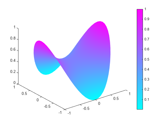
generateMesh(model,'GeometricOrder','linear','Hmax',0.1); u = pdenonlin(model,c,a,f); pdeplot(model,'XYData',u,'ZData',u)
Minimal Surface Problem Using [p,e,t] Mesh
Solve the minimal surface problem using the legacy approach for creating boundary conditions and geometry.
Create the geometry using the built-in circleg
function. Plot the geometry to see the edge labels.
g = @circleg; pdegplot(g,'EdgeLabels','on') axis equal
Create Dirichlet boundary conditions with value .Create the following file and save it on your MATLAB path.
function [qmatrix,gmatrix,hmatrix,rmatrix] = pdex2bound(p,e,u,time)
ne = size(e,2); % number of edges qmatrix = zeros(1,ne); gmatrix = qmatrix; hmatrix = zeros(1,2*ne); rmatrix = hmatrix;
for k = 1:ne x1 = p(1,e(1,k)); % x at first point in segment x2 = p(1,e(2,k)); % x at second point in segment xm = (x1 + x2)/2; % x at segment midpoint y1 = p(2,e(1,k)); % y at first point in segment y2 = p(2,e(2,k)); % y at second point in segment ym = (y1 + y2)/2; % y at segment midpoint switch e(5,k) case {1,2,3,4} hmatrix(k) = 1; hmatrix(k+ne) = 1; rmatrix(k) = x1^2; rmatrix(k+ne) = x2^2; end end
Set the coefficients and boundary conditions.
a = 0;
f = 0;
c = '1./sqrt(1+ux.^2+uy.^2)';
b = @pdex2bound;
Generate a mesh and solve the problem.
[p,e,t] = initmesh(g,'Hmax',0.1); u = pdenonlin(b,p,e,t,c,a,f); pdeplot(p,e,t,'XYData',u,'ZData',u)
Nonlinear Problem with 3-D Geometry
Solve a nonlinear 3-D problem with nontrivial geometry.
Import the geometry from the BracketWithHole.stl
file. Plot the geometry and face labels.
model = createpde(); importGeometry(model,'BracketWithHole.stl'); figure pdegplot(model,'FaceLabels','on','FaceAlpha',0.5) view(30,30) title('Bracket with Face Labels')
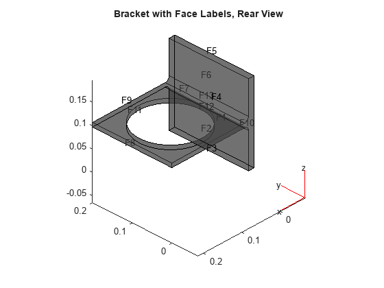
figure pdegplot(model,'FaceLabels','on','FaceAlpha',0.5) view(-134,-32) title('Bracket with Face Labels, Rear View')
Set a Dirichlet boundary condition with value 1000 on the back face, which is face 4. Set the large faces 1 and 7, and also the circular face 11, to have Neumann boundary conditions with value g = -10
. Do not set boundary conditions on the other faces. Those faces default to Neumann boundary conditions with value g = 0
.
applyBoundaryCondition(model,'Face',4,'u',1000); applyBoundaryCondition(model,'Face',[1,7,11],'g',-10);
Set the c
coefficient to 1, f
to 0.1, and a
to the nonlinear value '0.1 + 0.001*u.^2'
.
c = 1;
f = 0.1;
a = '0.1 + 0.001*u.^2';
Generate the mesh and solve the PDE. Start from the initial guess u0 = 1000
, which matches the value you set on face 4. Turn on the Report
option to observe the convergence during the solution.
generateMesh(model); u = pdenonlin(model,c,a,f,'U0',1000,'Report','on');
Iteration Residual Step size Jacobian: full 0 7.0647e-01 1 1.0525e-01 1.0000000 2 3.1238e-02 1.0000000 3 8.7268e-03 1.0000000 4 1.7657e-03 1.0000000 5 1.3879e-04 1.0000000 6 1.1079e-06 1.0000000
Plot the solution on the geometry boundary.
pdeplot3D(model,'ColorMapData',u)
Input Arguments
model
— PDE model
PDEModel
object
PDE model, specified as a PDEModel
object.
Example: model = createpde
c
— PDE coefficient
scalar | matrix | character vector | character array | string scalar | string vector | coefficient function
PDE coefficient, specified as a scalar, matrix, character vector, character array, string
scalar, string vector, or coefficient function. c
represents the c coefficient in the scalar PDE
or in the system of PDEs
Example: 'cosh(x+y.^2)'
Data Types: double
| char
| string
| function_handle
Complex Number Support: Yes
a
— PDE coefficient
scalar | matrix | character vector | character array | string scalar | string vector | coefficient function
PDE coefficient, specified as a scalar, matrix, character vector, character array, string
scalar, string vector, or coefficient function. a
represents the
a coefficient in the scalar PDE
or in the system of PDEs
Example: 2*eye(3)
Data Types: double
| char
| string
| function_handle
Complex Number Support: Yes
f
— PDE coefficient
scalar | matrix | character vector | character array | string scalar | string vector | coefficient function
PDE coefficient, specified as a scalar, matrix, character vector, character array, string
scalar, string vector, or coefficient function. f
represents the f coefficient in the scalar PDE
or in the system of PDEs
Example: char('sin(x)';'cos(y)';'tan(z)')
Data Types: double
| char
| string
| function_handle
Complex Number Support: Yes
b
— Boundary conditions
boundary matrix | boundary file
Boundary conditions, specified as a boundary matrix or boundary file. Pass a boundary file as a function handle or as a file name. A boundary matrix is generally an export from the PDE Modeler app.
Example: b = 'circleb1'
, b = "circleb1"
, or b =
@circleb1
Data Types: double
| char
| string
| function_handle
p
— Mesh points
matrix
Mesh points, specified as a 2-by-Np
matrix of points, where
Np
is the number of points in the mesh. For a description of the
(p
,e
,t
) matrices, see Mesh Data as [p,e,t] Triples.
Typically, you use the p
, e
, and t
data exported from the PDE Modeler app, or generated by initmesh
or refinemesh
.
Example: [p,e,t] = initmesh(gd)
Data Types: double
e
— Mesh edges
matrix
Mesh edges, specified as a 7
-by-Ne
matrix of edges,
where Ne
is the number of edges in the mesh. For a description of the
(p
,e
,t
) matrices, see Mesh Data as [p,e,t] Triples.
Typically, you use the p
, e
, and t
data exported from the PDE Modeler app, or generated by initmesh
or refinemesh
.
Example: [p,e,t] = initmesh(gd)
Data Types: double
t
— Mesh triangles
matrix
Mesh triangles, specified as a 4
-by-Nt
matrix of
triangles, where Nt
is the number of triangles in the mesh. For a
description of the (p
,e
,t
)
matrices, see Mesh Data as [p,e,t] Triples.
Typically, you use the p
, e
, and t
data exported from the PDE Modeler app, or generated by initmesh
or refinemesh
.
Example: [p,e,t] = initmesh(gd)
Data Types: double
Name-Value Arguments
Specify optional pairs of arguments as
Name1=Value1,...,NameN=ValueN
, where Name
is
the argument name and Value
is the corresponding value.
Name-value arguments must appear after other arguments, but the order of the
pairs does not matter.
Before R2021a, use commas to separate each name and value, and enclose
Name
in quotes.
Example: 'Jacobian','full'
Jacobian
— Approximation of Jacobian
'full'
(3-D
default) | 'fixed'
(2-D
default) | 'lumped'
Approximation of Jacobian, specified as
'full'
,
'fixed'
, or
'lumped'
.
'full'
means numerical evaluation of the full Jacobian based on the sparse version of thenumjac
function. 3-D geometry uses only'full'
, any other specification yields an error.'fixed'
specifies a fixed-point iteration matrix where the Jacobian is approximated by the stiffness matrix. This is the 2-D geometry default.'lumped'
specifies a “lumped” approximation as described in Nonlinear Equations. This approximation is based on the numerical differentiation of the coefficients.
Example: u =
pdenonlin(model,c,a,f,'Jacobian','full')
Data Types: char
| string
U0
— Initial solution guess
0 (default) | scalar | vector of characters | vector of numbers
Initial solution guess, specified as a scalar, a vector of characters, or a vector of numbers. A scalar specifies a constant initial condition for either a scalar or PDE system.
For systems of N
equations, and a mesh with Np
nodes, give a column vector with
N*Np
components. The nodes are either
model.Mesh.Nodes
, or the p
data from
initmesh
or meshToPet
. See Mesh Data as [p,e,t] Triples.
The first
Np
elements contain the values of component 1, where
the value of element k
corresponds to node p(k)
. The
next Np
points contain the values of component 2, etc. It
can be convenient to first represent the initial
conditions u0
as an
Np
-by-N
matrix, where the first column contains entries
for component 1, the second column contains
entries for component 2, etc. The final
representation of the initial conditions is
u0(:)
.
Example: u =
pdenonlin(model,c,a,f,'U0','x.^2-y.^2')
Data Types: double
| char
| string
Complex Number Support: Yes
Tol
— Residual size at termination
1e-4 (default) | positive scalar
Residual size at termination, specified as a
positive scalar. pdenonlin
iterates until the residual size is less than
'Tol'
.
Example: u =
pdenonlin(model,c,a,f,'Tol',1e-6)
Data Types: double
MaxIter
— Maximum number of Gauss-Newton iterations
25
(default) | positive integer
Maximum number of Gauss-Newton iterations, specified as a positive integer.
Example: u =
pdenonlin(model,c,a,f,'MaxIter',12)
Data Types: double
MinStep
— Minimum damping of search direction
1/2^16
(default) | positive scalar
Minimum damping of search direction, specified as a positive scalar.
Example: u =
pdenonlin(model,c,a,f,'MinStep',1e-3)
Data Types: double
Report
— Print convergence information
'off'
(default) | 'on'
Print convergence information, specified as
'off'
or
'on'
.
Example: u =
pdenonlin(model,c,a,f,'Report','on')
Data Types: char
| string
Norm
— Residual norm
Inf
(default) | p value for Lp
norm | 'energy'
Residual norm, specified as the
p
value for
Lp norm, or as
'energy'
. p
can be any positive real value,
Inf
, or
-Inf
. The p
norm of a vector v
is
sum(abs(v)^p)^(1/p)
. See
norm
.
Example: u =
pdenonlin(model,c,a,f,'Norm',2)
Data Types: double
| char
| string
Output Arguments
u
— PDE solution
vector
PDE solution, returned as a vector.
If the PDE is scalar, meaning only one equation, then
u
is a column vector representing the solution u at each node in the mesh.u(i)
is the solution at thei
th column ofmodel.Mesh.Nodes
or thei
th column ofp
.If the PDE is a system of N > 1 equations, then
u
is a column vector with N*Np
elements, whereNp
is the number of nodes in the mesh. The firstNp
elements ofu
represent the solution of equation 1, then nextNp
elements represent the solution of equation 2, etc.
To obtain the solution at an arbitrary point in the geometry,
use pdeInterpolant
.
res
— Norm of Newton step residuals
scalar
Norm of Newton step residuals, returned as a scalar. For information about the algorithm, see Nonlinear Equations.
Tips
If the Newton iteration does not converge,
pdenonlin
displays the error messageToo many iterations
orStepsize too small
.If the initial guess produces matrices containing
NaN
orInf
elements,pdenonlin
displays the error messageUnsuitable initial guess U0 (default: U0 = 0)
.If you have very small coefficients, or very small geometric dimensions,
pdenonlin
can fail to converge, or can converge to an incorrect solution. If so, you can sometimes obtain better results by scaling the coefficients or geometry dimensions to be of order one.
Algorithms
Nonlinear Equations
The basic idea is to use Gauss-Newton iterations to solve the nonlinear equations. Say you are trying to solve the equation
r(u) = –∇ · (c(u)∇u) + a(u)u - f(u) = 0.
In the FEM setting you solve the weak form of r(u) = 0. Set as usual
where x represents a 2-D or 3-D point. Then multiply the equation by an arbitrary test function ϕi, integrate on the domain Ω, and use Green's formula and the boundary conditions to obtain
which has to hold for all indices i.
The residual vector ρ(U) can be easily computed as
ρ(U) = (K + M + Q)U – (F + G)
where the matrices K, M, Q and the vectors F and G are produced by assembling the problem
–∇ · (c(U)∇u) + a(U)u = f(U).
Assume that you have a guess U(n) of the solution. If U(n) is close enough to the exact solution, an improved approximation U(n+1) is obtained by solving the linearized problem
where is a positive number. (It is not necessary that ρ(U) = 0 have a solution even if ρ(u) = 0 has.) In this case, the Gauss-Newton iteration tends to be the minimizer of the residual, i.e., the solution of minU .
It is well known that for sufficiently small
and
is called a descent direction for , where is the L2-norm. The iteration is
where ≤ 1 is chosen as large as possible such that the step has a reasonable descent.
The Gauss-Newton method is local, and convergence is assured only when U(0) is close enough to the solution. In general, the first guess may be outside the region of convergence. To improve convergence from bad initial guesses, a damping strategy is implemented for choosing α, the Armijo-Goldstein line search. It chooses the largest damping coefficient α out of the sequence 1, 1/2, 1/4, . . . such that the following inequality holds:
which guarantees a reduction of the residual norm by at least 1 – /2. Each step of the line-search algorithm requires an evaluation of the residual .
An important point of this strategy is that when U(n) approaches the solution, then →1 and thus the convergence rate increases. If there is a solution to ρ(U) = 0, the scheme ultimately recovers the quadratic convergence rate of the standard Newton iteration.
Closely related to the preceding problem is the choice of the initial guess U(0). By default, the solver sets U(0) and then assembles the FEM matrices K and F and computes
U(1) = K–1F
The damped Gauss-Newton iteration is then started with U(1), which should be a better guess than U(0). If the boundary conditions do not depend on the solution u, then U(1) satisfies them even if U(0) does not. Furthermore, if the equation is linear, then U(1) is the exact FEM solution and the solver does not enter the Gauss-Newton loop.
There are situations where U(0) = 0 makes no sense or convergence is impossible.
In some situations you may already have a good approximation and the nonlinear solver can be started with it, avoiding the slow convergence regime. This idea is used in the adaptive mesh generator. It computes a solution on a mesh, evaluates the error, and may refine certain triangles. The interpolant of is a very good starting guess for the solution on the refined mesh.
In general the exact Jacobian
is not available. Approximation of Jn by finite differences in the following way is expensive but feasible. The ith column of Jn can be approximated by
which implies the assembling of the FEM matrices for the triangles containing grid point i. A very simple approximation to Jn, which gives a fixed point iteration, is also possible as follows. Essentially, for a given U(n), compute the FEM matrices K and F and set
U(n+1) = K–1F.
This is equivalent to approximating the Jacobian with the stiffness matrix. Indeed, since ρ(U(n)) = KU(n) – F, putting Jn = K yields
In many cases the convergence rate is slow, but the cost of each iteration is cheap.
The Partial Differential Equation Toolbox™ nonlinear solver also provides for a compromise between the two extremes. To compute the derivative of the mapping U→KU, proceed as follows. The a term has been omitted for clarity, but appears again in the final result.
The first integral term is nothing more than Ki,j.
The second term is “lumped,” i.e., replaced by a diagonal matrix that contains the row sums. Since Σjϕj = 1, the second term is approximated by
which is the ith component of K(c')U, where K(c') is the stiffness matrix associated with the coefficient ∂c/∂u rather than c. The same reasoning can be applied to the derivative of the mapping U→MU. The derivative of the mapping U→ –F is exactly
which is the mass matrix associated with the coefficient ∂f/∂u. Thus the Jacobian of the residual ρ(U) is approximated by
where the differentiation is with respect to u, K and M designate stiffness and mass matrices, and their indices designate the coefficients with respect to which they are assembled. At each Gauss-Newton iteration, the nonlinear solver assembles the matrices corresponding to the equations
and then produces the approximate Jacobian. The differentiations of the coefficients are done numerically.
In the general setting of elliptic systems, the boundary conditions are appended to the stiffness matrix to form the full linear system:
where the coefficients of and may depend on the solution . The “lumped” approach approximates the derivative mapping of the residual by
The nonlinearities of the boundary conditions and the dependencies of the coefficients on the derivatives of are not properly linearized by this scheme. When such nonlinearities are strong, the scheme reduces to the fix-point iteration and may converge slowly or not at all. When the boundary conditions are linear, they do not affect the convergence properties of the iteration schemes. In the Neumann case they are invisible (H is an empty matrix) and in the Dirichlet case they merely state that the residual is zero on the corresponding boundary points.
Version History
Introduced before R2006aR2016a: Not recommended
pdenonlin
is not recommended. Use solvepde
instead. There are no plans to remove
pdenonlin
.
See Also
MATLAB Command
You clicked a link that corresponds to this MATLAB command:
Run the command by entering it in the MATLAB Command Window. Web browsers do not support MATLAB commands.
Select a Web Site
Choose a web site to get translated content where available and see local events and offers. Based on your location, we recommend that you select: .
You can also select a web site from the following list
How to Get Best Site Performance
Select the China site (in Chinese or English) for best site performance. Other MathWorks country sites are not optimized for visits from your location.
Americas
- América Latina (Español)
- Canada (English)
- United States (English)
Europe
- Belgium (English)
- Denmark (English)
- Deutschland (Deutsch)
- España (Español)
- Finland (English)
- France (Français)
- Ireland (English)
- Italia (Italiano)
- Luxembourg (English)
- Netherlands (English)
- Norway (English)
- Österreich (Deutsch)
- Portugal (English)
- Sweden (English)
- Switzerland
- United Kingdom (English)
Asia Pacific
- Australia (English)
- India (English)
- New Zealand (English)
- 中国
- 日本Japanese (日本語)
- 한국Korean (한국어)