Monitor During Parallel Optimizations with parfeval

This example shows how to perform multiple optimizations in parallel with parfeval and monitor the progress of the optimizations on the client.

You can use a DataQueue object to send progress data from workers to the client during computations on a parallel pool. If your optimization function supports the OutputFcn option, you can specify an output function that sends progress data to the client at each iteration with the DataQueue. You can also use a DataQueue with parallel language features such as parfor, parfeval and spmd.

The example shows how to:

• Perform several optimizations of the Rosenbrock function [1] from different starting points, in parallel.

• Monitor the progress of the optimizations on the client by using a custom plot function.

Set Up Parallel Environment

Start a parallel pool of process workers on the local machine.

parpool("Processes");

Starting parallel pool (parpool) using the 'Processes' profile ...
Connected to parallel pool with 6 workers.

Define Problem

The problem is to minimize the two-variable Rosenbrock function, $f\left(x\right)=100{\left(x_2-x_1^2\right)}^2+{\left(1-x_1\right)}^2$, subject to the constraint $x_1^2+x_2^2\le 1$. The constraint defines a unit disk centered at the origin. In this example, you solve the problem from multiple starting points inside the unit disk and monitor the progress of each optimization.

Define the objective function and the nonlinear constraint function.

fun = @(x)(100*(x(2) - x(1)^2)^2 + (1 - x(1))^2);
nonlcon = @(x) deal(x(1)^2 + x(2)^2 - 1,[]);

Specify multiple starting points for performing the minimization. Use symmetry pairs to visualize how the trajectories of the optimizations can differ due to the symmetry of the curved valley of the Rosenbrock function.

x0 = [-0.5 0.2;
    0.5 -0.2;
    -0.2 0.5;
    0.2 -0.5];

Set Up Progress Visualization

Create a figure with one animated line plot per start point. To create the figure, use the preparePlots helper function, which is defined at the end of the example.

numStartPoints = size(x0,1);
[fig,hAx,hLines] = preparePlots(numStartPoints);

Create a DataQueue object to send the solver progress data from the workers to the client.

progressQueue = parallel.pool.DataQueue;

To visualize the progress updates that the workers send to the DataQueue, use afterEach to call the plotSolverProgress helper function each time a worker sends data. The plotSolverProgress helper function is defined at the end of the example.

plotFcn = @(data) plotSolverProgress(hAx,hLines,data{:});
afterEach(progressQueue,plotFcn);

Run and Monitor Optimizations in Parallel

Preallocate a vector of parallel.FevalFuture objects to hold results for the parfeval computations.

solverFutures(1:numStartPoints) = parallel.FevalFuture;

Using a for-loop, launch one parfeval computation per starting point to run fmincon in parallel. For each computation, define an OutputFcn that uses the sendSolverProgress helper function to send iteration progress back to the client through a DataQueue. An anonymous function passes the computation index and DataQueue object to the workers. Each parfeval call runs fmincon with the specified input arguments and options and requests four outputs. parfeval returns Future objects that let you collect results asynchronously as each computation finishes. The sendSolverProgress helper function is defined at the end of the example.

for idx = 1:numStartPoints
    outFcn = @(x,v,s) sendSolverProgress(x,v,s,idx,progressQueue);
    opts = optimoptions("fmincon",Display="off",OutputFcn=outFcn);
    solverFutures(idx) = parfeval(@fmincon,4,fun,x0(idx,:), ...
        [],[],[],[],[],[],nonlcon,opts);
end

Set the figure to visible to see the trajectories of each optimization running on the workers.

fig.Visible = "on";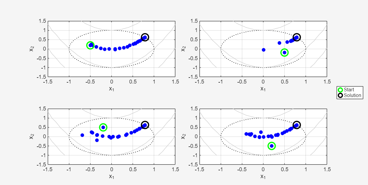

parfeval does not block MATLAB®, so you can continue working while the computations take place. The workers compute in parallel and send progress data through the DataQueue at each iteration.

If you want to block MATLAB until parfeval completes, use the wait function on the Future objects. Using the wait function is useful when subsequent code depends on the completion of parfeval.

wait(solverFutures);

Collect and Display Results

After parfeval finishes the computations, wait finishes and you can execute more code.

Retrieve the results of the optimizations by using the fetchOutputs function.

[sol,fval,eflag,output] = fetchOutputs(solverFutures);

Display the number of iterations required to solve the problem from the different starting points in a table.

numIterations = [output.iterations]';
t = table(x0,numIterations, ...
    VariableNames=["Starting Points","Iterations"]);
disp(t)

    Starting Points    Iterations
    _______________    __________

     -0.5     0.2          35    
      0.5    -0.2          24    
     -0.2     0.5          35    
      0.2    -0.5          39    

The results show that the number of iterations required for convergence depends on the starting point. Starting points that are closer to the curved valley of the Rosenbrock function converge in fewer iterations, while starting points farther from the valley require more iterations to reach the solution.

References

[1] Rosenbrock, H. H. “An Automatic Method for Finding the Greatest or Least Value of a Function.” The Computer Journal 3, no. 3 (1960): 175–84. https://doi.org/10.1093/comjnl/3.3.175.

Helper Functions

sendSolverProgress Function

The sendSolverProgress function sends the current solver state and iteration information to the client via a DataQueue object. You must call the sendSolverProgress function as an OutputFcn on each solver iteration. For more information about the structure of an output function, see Output Function and Plot Function Syntax (Optimization Toolbox).

function stop = sendSolverProgress(x,optimValues,state,idx,queue)
stop = false;
send(queue,{idx,x,optimValues,state});
pause(0.5); % Simulate an expensive function by pausing
end

plotSolverProgress Function

The plotSolverProgress function plots the progress of an optimization as it runs. The function uses the state input to perform different actions at the start of the optimization, during iterations, and at completion:

• On "init": Initializes the plot for the current starting point. Marks the start and solution locations and titles the axes with the starting point.

• On "iter": Appends the current iterate to an animated line to show the trajectory of the solver.

• On "done": Adds a subtitle summarizing the final point and releases the hold state on the axes.

For more information about the structure of plot functions, see Output Function and Plot Function Syntax (Optimization Toolbox).

function stop = plotSolverProgress(hAx,hLines,idx,x,optimValues,state)
%  Plot solver trajectories for each starting point.
stop = false;
ax = hAx(idx);
switch state
    case "init"
        hold(ax,"on");
        x1 = x(1);
        x2 = x(2);
        z1 = optimValues.fval;
        title(ax,sprintf("Starting Point [%.1f,%.1f]",x1,x2))
        pStart = plot3(ax,x1,x2,z1,"go",MarkerSize=12,LineWidth=2);
        pSol = plot3(ax,0.79,0.62,0,"ko",MarkerSize=12,LineWidth=2);
        if idx == 1
        lgd = legend([pStart,pSol],["Start","Solution"]);
        lgd.Layout.Tile = "east";
        end
        drawnow limitrate nocallbacks;
    case "iter"
        al = hLines(idx);
        x1 = x(1);
        x2 = x(2);
        z1 = optimValues.fval;
        addpoints(al,x1,x2,z1);
        ax.SortMethod = "childorder";
        drawnow limitrate nocallbacks;
    case "done"
        subtitle(ax,sprintf("Local minimum found [%.2f,%.2f]", ...
            x(1),x(2)));
        hold(ax,"off");
end
end

preparePlots Function

The preparePlots function creates figure, axes, and animated line objects for visualizing the optimization progress. Specifically, the function:

• Builds a tiled layout and returns handles to the axes

• Precomputes and displays the Rosenbrock objective contours over a grid in each tile

• Draws the unit-disk boundary $x_1^2+x_2^2-1=0$ as a reference

• Creates one animated line per tile and returns the handles for incremental trajectory updates during optimization

function [fig,hAx,lineHdls] = preparePlots(numPlots)
fig = figure(Name="Optimization Progress",Visible="off");
t = tiledlayout(fig,"flow",TileSpacing="tight");
hAx = gobjects(1,numPlots);
lineHdls = gobjects(1,numPlots);
xx = -3:.2:3;
yy = -1:.2:3;
[xx,yy] = meshgrid(xx,yy);
zz = 100*(yy-xx.^2).^2+(1-xx).^2;
for idx=1:numPlots
    ax = nexttile(t);
    axis(ax,"equal");
    box(ax,"on");
    th = linspace(0,2*pi,400);
    plot(ax,cos(th),sin(th),"k:");     
    xlabel("x_{1}");
    ylabel("x_{2}");
    zlabel("Rosenbrock Value");
    xlim(ax,[-1.5 1.5])
    ylim(ax,[-1.5 1.5])
    grid on 
    hold(ax,"on");
    [~,contHndl] = contour3(ax,xx,yy,zz,[100,500],"k");
    contHndl.Color = [0.8,0.8,0.8];
    hold(ax,"off");
    hAx(idx) = ax;
    lineHdls(idx) = animatedline(ax,NaN,NaN,NaN, ...
        Color="none",Marker="o",MarkerFaceColor="b");
end
end