地上ビークルの位置と向きの推定

この例では、慣性測定ユニット (IMU) と全地球測位システム (GPS) 受信機からのデータを融合させて、地上ビークルの位置と向きを推定する方法を説明します。

シミュレーションの設定

サンプリングレートを設定します。典型的なシステムでは、IMU 内の加速度計およびジャイロスコープは、比較的高いサンプルレートで動作します。これらのセンサーからのデータをフュージョンアルゴリズムで処理することは、それほど複雑ではありません。逆に、GPS は比較的低いサンプルレートで動作するため、その処理に関連する複雑度は高くなります。このフュージョンアルゴリズムでは、GPS のサンプルは低いレートで処理され、加速度計とジャイロスコープのサンプルは共に同じ高いレートで処理されます。

この構成をシミュレートするために、IMU (加速度計とジャイロスコープ) は 100 Hz でサンプリングされ、GPS は 10 Hz でサンプリングされます。

imuFs = 100;
gpsFs = 10;

% Define where on the Earth this simulation takes place using latitude, 
% longitude, and altitude (LLA) coordinates.
localOrigin = [42.2825 -71.343 53.0352];

% Validate that the |gpsFs| divides |imuFs|. This allows the sensor sample
% rates to be simulated using a nested for loop without complex sample rate
% matching.

imuSamplesPerGPS = (imuFs/gpsFs);
assert(imuSamplesPerGPS == fix(imuSamplesPerGPS), ...
    'GPS sampling rate must be an integer factor of IMU sampling rate.');

フュージョンフィルター

IMU と GPS の測定を融合するフィルターを作成します。フュージョンフィルターは、拡張カルマンフィルターを使用して、向き (四元数として)、位置、速度、およびセンサーバイアスを追跡します。

insfilterNonholonomic オブジェクトには、predict と fusegps の 2 つのメインメソッドがあります。predict メソッドは、IMU から加速度計およびジャイロスコープのサンプルを入力として取ります。加速度計とジャイロスコープがサンプリングされるたびに、predict メソッドを呼び出します。このメソッドは、加速度計とジャイロスコープに基づいて、1 タイムステップ先の状態を予測します。拡張カルマンフィルターの誤差の共分散は、このステップで更新されます。

fusegps メソッドは、GPS のサンプルを入力として取ります。このメソッドは、さまざまなセンサー入力を不確かさに従って重み付けするカルマンゲインを計算することにより、GPS サンプルに基づいてフィルターの状態を更新します。誤差の共分散はこのステップでも更新され、今回はカルマンゲインも使用されます。

insfilterNonholonomic オブジェクトには、IMUSampleRate と DecimationFactor という 2 つのメインプロパティがあります。地上ビークルには、地面から飛び上がることも地面でスライドすることもないと想定する、2 つの速度制約があります。これらの制約は、拡張カルマンフィルターの更新方程式を使用して適用されます。これらの更新は、IMUSampleRate/DecimationFactor Hz のレートでフィルターの状態に適用されます。

gndFusion = insfilterNonholonomic('ReferenceFrame', 'ENU', ...
    'IMUSampleRate', imuFs, ...
    'ReferenceLocation', localOrigin, ...
    'DecimationFactor', 2);

地上ビークルの軌跡の作成

waypointTrajectory オブジェクトは、指定されたサンプリングレート、ウェイポイント、到着時間、および向きに基づいて姿勢を計算します。地上ビークルの円形軌跡のパラメーターを指定します。

% Trajectory parameters
r = 8.42; % (m)
speed = 2.50; % (m/s)
center = [0, 0]; % (m)
initialYaw = 90; % (degrees)
numRevs = 2;

% Define angles theta and corresponding times of arrival t.
revTime = 2*pi*r / speed;
theta = (0:pi/2:2*pi*numRevs).';
t = linspace(0, revTime*numRevs, numel(theta)).';

% Define position.
x = r .* cos(theta) + center(1);
y = r .* sin(theta) + center(2);
z = zeros(size(x));
position = [x, y, z];

% Define orientation.
yaw = theta + deg2rad(initialYaw);
yaw = mod(yaw, 2*pi);
pitch = zeros(size(yaw));
roll = zeros(size(yaw));
orientation = quaternion([yaw, pitch, roll], 'euler', ...
    'ZYX', 'frame');

% Generate trajectory.
groundTruth = waypointTrajectory('SampleRate', imuFs, ...
    'Waypoints', position, ...
    'TimeOfArrival', t, ...
    'Orientation', orientation);

% Initialize the random number generator used to simulate sensor noise.
rng('default');

GPS 受信機

指定のサンプルレートと参照場所で GPS を設定します。他のパラメーターは、出力信号内のノイズの性質を制御します。

gps = gpsSensor('UpdateRate', gpsFs, 'ReferenceFrame', 'ENU');
gps.ReferenceLocation = localOrigin;
gps.DecayFactor = 0.5;                % Random walk noise parameter 
gps.HorizontalPositionAccuracy = 1.0;   
gps.VerticalPositionAccuracy =  1.0;
gps.VelocityAccuracy = 0.1;

IMU センサー

通常、地上ビークルは姿勢の推定に 6 軸の IMU センサーを使用します。IMU センサーをモデル化するには、加速度計とジャイロスコープを含む IMU センサーモデルを定義します。実際のアプリケーションでは、2 つのセンサーは、単一の集積回路によることも別々の回路に由来することもあります。ここで設定するプロパティ値は、低コストの MEMS センサーに典型的なものです。

imu = imuSensor('accel-gyro', ...
    'ReferenceFrame', 'ENU', 'SampleRate', imuFs);

% Accelerometer
imu.Accelerometer.MeasurementRange =  19.6133;
imu.Accelerometer.Resolution = 0.0023928;
imu.Accelerometer.NoiseDensity = 0.0012356;

% Gyroscope
imu.Gyroscope.MeasurementRange = deg2rad(250);
imu.Gyroscope.Resolution = deg2rad(0.0625);
imu.Gyroscope.NoiseDensity = deg2rad(0.025);

`insfilterNonholonomic` の状態の初期化

以下の状態があります。

States                            Units    Index
Orientation (quaternion parts)             1:4  
Gyroscope Bias (XYZ)              rad/s    5:7  
Position (NED)                    m        8:10 
Velocity (NED)                    m/s      11:13
Accelerometer Bias (XYZ)          m/s^2    14:16

フィルターが短時間で適切な回答に収束するよう、フィルターの状態の初期化を補助するためにグラウンドトゥルースが使用されます。

% Get the initial ground truth pose from the first sample of the trajectory
% and release the ground truth trajectory to ensure the first sample is not 
% skipped during simulation.
[initialPos, initialAtt, initialVel] = groundTruth();
reset(groundTruth);

% Initialize the states of the filter
gndFusion.State(1:4) = compact(initialAtt).';
gndFusion.State(5:7) = imu.Gyroscope.ConstantBias;
gndFusion.State(8:10) = initialPos.';
gndFusion.State(11:13) = initialVel.';
gndFusion.State(14:16) = imu.Accelerometer.ConstantBias;

`insfilterNonholonomic` の分散の初期化

測定ノイズは、どれだけのノイズが GPS の読み取り値を破損しているかを、gpsSensor パラメーターとビークルの動的モデルにある不確かさの程度に基づいて記述します。

プロセスノイズは、フィルター方程式が状態の進展をどの程度よく説明しているかを記述します。プロセスノイズは、パラメーターのスイープを使用してフィルターからの位置と向きの推定を一緒に最適化することにより、経験的に決定されます。

% Measurement noises
Rvel = gps.VelocityAccuracy.^2;
Rpos = gps.HorizontalPositionAccuracy.^2;

% The dynamic model of the ground vehicle for this filter assumes there is
% no side slip or skid during movement. This means that the velocity is 
% constrained to only the forward body axis. The other two velocity axis 
% readings are corrected with a zero measurement weighted by the 
% |ZeroVelocityConstraintNoise| parameter.
gndFusion.ZeroVelocityConstraintNoise = 1e-2;

% Process noises
gndFusion.GyroscopeNoise = 4e-6;
gndFusion.GyroscopeBiasNoise = 4e-14;
gndFusion.AccelerometerNoise = 4.8e-2;
gndFusion.AccelerometerBiasNoise = 4e-14;

% Initial error covariance
gndFusion.StateCovariance = 1e-9*eye(16);

スコープの初期化

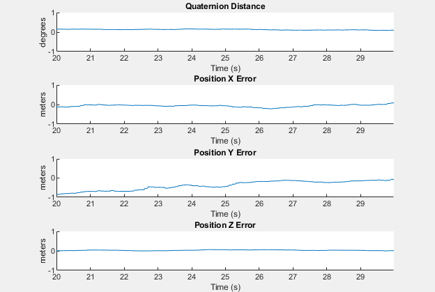
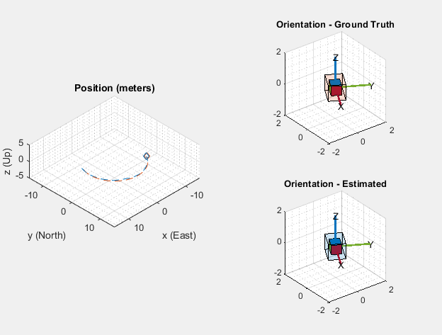
HelperScrollingPlotter スコープを使うと、変数の経時的なプロットが可能になります。ここでは、姿勢の誤差を追跡するために使用します。HelperPoseViewer スコープを使うと、フィルター推定値とグラウンドトゥルース姿勢を 3 次元で可視化できます。スコープによってシミュレーション速度は低下する場合があります。スコープを無効にするには、対応する論理変数を false に設定します。

useErrScope = true; % Turn on the streaming error plot
usePoseView = true;  % Turn on the 3D pose viewer

if useErrScope
    errscope = HelperScrollingPlotter( ...
            'NumInputs', 4, ...
            'TimeSpan', 10, ...
            'SampleRate', imuFs, ...
            'YLabel', {'degrees', ...
            'meters', ...
            'meters', ...
            'meters'}, ...
            'Title', {'Quaternion Distance', ...
            'Position X Error', ...
            'Position Y Error', ...
            'Position Z Error'}, ...
            'YLimits', ...
            [-1, 1
             -1, 1
             -1, 1
             -1, 1]);
end

if usePoseView
    viewer = HelperPoseViewer( ...
        'XPositionLimits', [-15, 15], ...
        'YPositionLimits', [-15, 15], ...
        'ZPositionLimits', [-5, 5], ...
        'ReferenceFrame', 'ENU');
end

シミュレーションループ

メインのシミュレーションループは、for ループが入れ子になっている while ループです。while ループは、GPS 測定レートである gpsFs で実行されます。入れ子になった for ループは、IMU サンプルレートである imuFs で実行されます。スコープは IMU サンプルレートで更新されます。

totalSimTime = 30; % seconds

% Log data for final metric computation.
numsamples = floor(min(t(end), totalSimTime) * gpsFs);
truePosition = zeros(numsamples,3);
trueOrientation = quaternion.zeros(numsamples,1);
estPosition = zeros(numsamples,3);
estOrientation = quaternion.zeros(numsamples,1);

idx = 0;

for sampleIdx = 1:numsamples
    % Predict loop at IMU update frequency.
    for i = 1:imuSamplesPerGPS
        if ~isDone(groundTruth)
            idx = idx + 1;
            
            % Simulate the IMU data from the current pose.
            [truePosition(idx,:), trueOrientation(idx,:), ...
                trueVel, trueAcc, trueAngVel] = groundTruth();
            [accelData, gyroData] = imu(trueAcc, trueAngVel, ...
                trueOrientation(idx,:));
            
            % Use the predict method to estimate the filter state based
            % on the accelData and gyroData arrays.
            predict(gndFusion, accelData, gyroData);
            
            % Log the estimated orientation and position.
            [estPosition(idx,:), estOrientation(idx,:)] = pose(gndFusion);
            
            % Compute the errors and plot.
            if useErrScope
                orientErr = rad2deg( ...
                    dist(estOrientation(idx,:), trueOrientation(idx,:)));
                posErr = estPosition(idx,:) - truePosition(idx,:);
                errscope(orientErr, posErr(1), posErr(2), posErr(3));
            end

            % Update the pose viewer.
            if usePoseView
                viewer(estPosition(idx,:), estOrientation(idx,:), ...
                    truePosition(idx,:), trueOrientation(idx,:));
            end
        end
    end
    
    if ~isDone(groundTruth)
        % This next step happens at the GPS sample rate.
        % Simulate the GPS output based on the current pose.
        [lla, gpsVel] = gps(truePosition(idx,:), trueVel);

        % Update the filter states based on the GPS data.
        fusegps(gndFusion, lla, Rpos, gpsVel, Rvel);
    end
end

MATLAB figure

誤差メトリクスの計算

位置と向きは、シミュレーション全体を通してログに記録されました。ここで、位置と向きの両方についてエンドツーエンドの平方根平均二乗誤差を計算します。

posd = estPosition - truePosition;

% For orientation, quaternion distance is a much better alternative to
% subtracting Euler angles, which have discontinuities. The quaternion
% distance can be computed with the |dist| function, which gives the
% angular difference in orientation in radians. Convert to degrees for
% display in the command window.

quatd = rad2deg(dist(estOrientation, trueOrientation));

% Display RMS errors in the command window.
fprintf('\n\nEnd-to-End Simulation Position RMS Error\n');

End-to-End Simulation Position RMS Error

msep = sqrt(mean(posd.^2));
fprintf('\tX: %.2f , Y: %.2f, Z: %.2f   (meters)\n\n', msep(1), ...
    msep(2), msep(3));

	X: 1.16 , Y: 0.98, Z: 0.03   (meters)

fprintf('End-to-End Quaternion Distance RMS Error (degrees) \n');

End-to-End Quaternion Distance RMS Error (degrees)

fprintf('\t%.2f (degrees)\n\n', sqrt(mean(quatd.^2)));

	0.11 (degrees)