radiusregion
Syntax
Description
radiusregion( creates a filled circular
region, or annulus, between the two specified radii in the current
(polar) axes. To create one filled region, specify r1,r2)r1 and
r2 as scalars. To create multiple filled regions, specify
r1 and r2 as vectors of the same length.
radiusregion(___,
specifies properties for the region using one or more name-value arguments. If you create
multiple regions, the property values apply to all of the regions. Specify the name-value
arguments after all other inputs. For example, create a yellow radius region using
Name=Value)radiusregion(5,10,FaceColor="yellow"). For a list of properties, see
PolarRegion Properties.
radiusregion( specifies
the target polar axes for the filled region. Specify pax,___)pax as the first
argument in any of the previous syntaxes.
pr = radiusregion(___) returns one or more
PolarRegion objects. Use pr to set properties of the
filled regions after creating them. For a list of properties, see PolarRegion Properties.
Examples
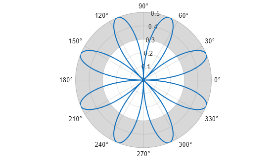
Create a polar plot and add a radius region that has an inner boundary of r=0.3 and an outer boundary of r=0.5.
% Create polar plot
theta = 0:0.01:2*pi;
rho = sin(2*theta).*cos(2*theta);
polarplot(theta,rho,LineWidth=1.5)

% Create filled region
r1 = 0.3;
r2 = 0.5;
radiusregion(r1,r2)
Change the theta-axis units to radians by setting the ThetaAxisUnits property.
pax = gca;
pax.ThetaAxisUnits = "radians";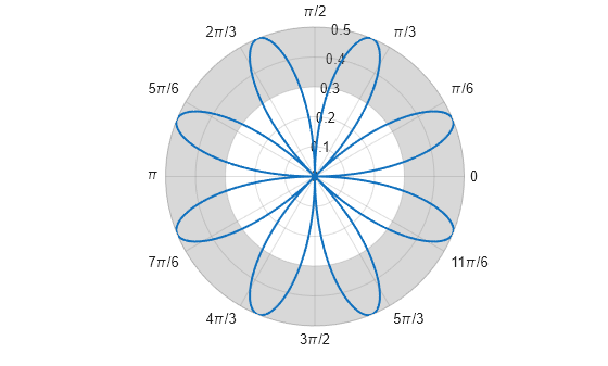
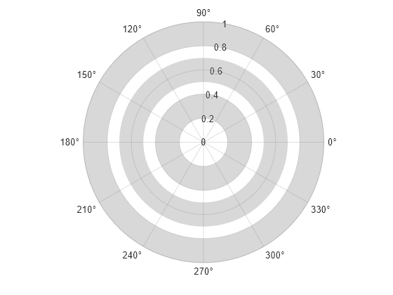
Create three concentric filled regions by specifying the bounding radii as three-element vectors.
r1 = [0.2 0.5 0.8];
r2 = [0.4 0.7 1];
radiusregion(r1,r2)

Alternatively, specify one 2-by-3 matrix of radius values.
figure
R = [0.2 0.5 0.8; 0.4 0.7 1];
radiusregion(R)
You can specify PolarRegion properties, such as face color and boundary line width and color, by specifying one or more name-value arguments when you call radiusregion. Alternatively, you can set properties of the PolarRegion object after creating it.
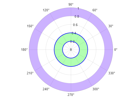
For example, create two green radius regions. Specify an output argument to store the PolarRegion objects so that you can modify them later.
r1 = [0.2 0.8];
r2 = [0.4 1];
rr = radiusregion(r1,r2,FaceColor="g");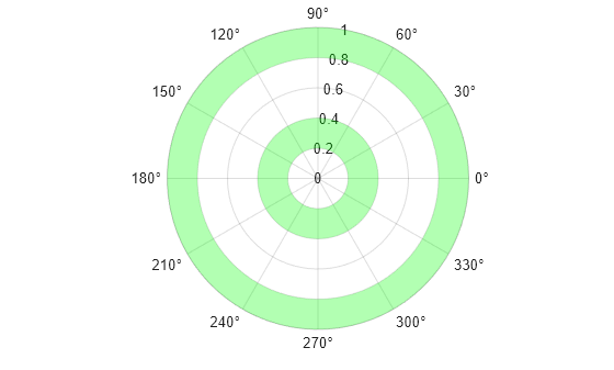
Change the color of the outer region to a shade of purple by specifying the FaceColor property as a hexadecimal color code. Then display thick boundary lines around the inner region by setting the EdgeColor property to a value other than "none" and setting the LineWidth property to 1.5.
% Set color of outer region
rr(2).FaceColor = "#5500FF";

% Set boundary color and line thickness
rr(1).EdgeColor = "b";
rr(1).LineWidth = 1.5;
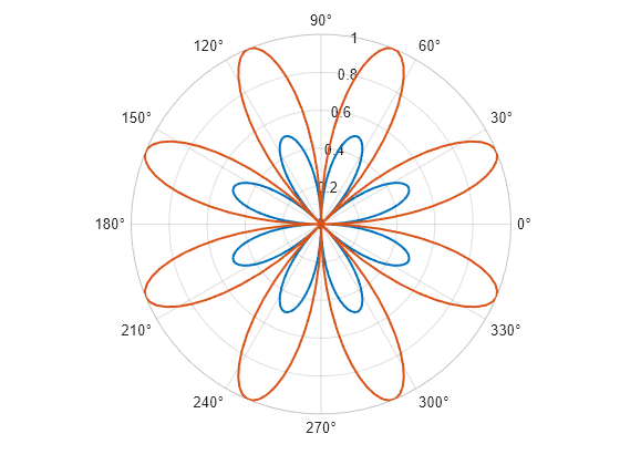
Plot a blue and a red rose.
theta = linspace(0,2*pi,200);
rho1 = sin(2*theta).*cos(2*theta);
rho2 = 2*sin(2*theta).*cos(2*theta);

% Blue rose
rose1 = polarplot(theta,rho1,LineWidth=1.5);
hold on

% Red rose
rose2 = polarplot(theta,rho2,LineWidth=1.5);
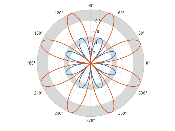
Create radius regions that highlight the tips of the rose petals.
r1 = 0.4;
r2 = 0.5;
region1 = radiusregion(r1,r2);

r3 = 0.8;
r4 = 1;
region2 = radiusregion(r3,r4);
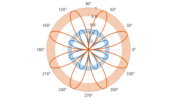
Match the color of each radius region to the corresponding rose by setting the SeriesIndex property of the region to the SeriesIndex property of the rose.
region1.SeriesIndex = rose1.SeriesIndex;
region2.SeriesIndex = rose2.SeriesIndex;
To move a radius region on top of a plot, set the Layer property of the PolarRegion object to "top". For example, plot a polar rose and add a radius region. When you create the radius region, specify a custom face color and transparency value so that you can see that the rose is on top of the radius region.
% Plot polar rose
theta = 0:0.01:2*pi;
rho = sin(2*theta).*cos(2*theta);
polarplot(theta,rho,LineWidth=1.5)

% Add radius region
r1 = 0.2;
r2 = 0.3;
rr = radiusregion(r1,r2,FaceColor=[0.8 0.8 0.8],FaceAlpha=0.7);
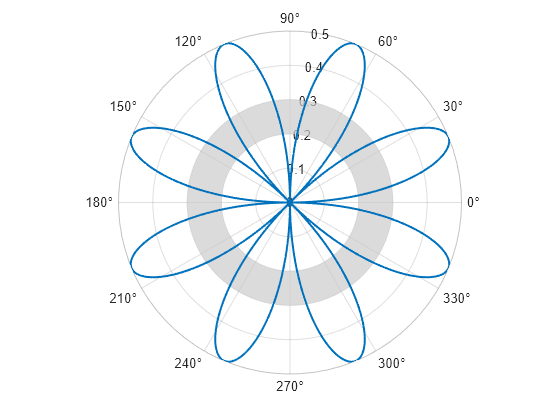
Move the radius region on top of the rose by setting the Layer property to "top".
rr.Layer = "top";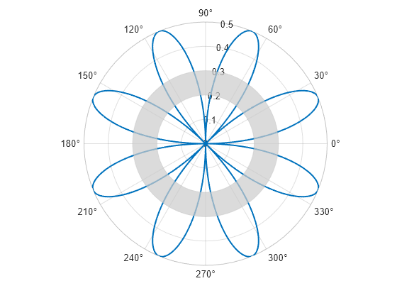
To create radius regions in different polar axes within the same figure, create a tiled chart layout. In this case, create two axes that each contain a radius region.
Use the tiledlayout function to create a 1-by-2 tiled chart layout t. Use the polaraxes function to create each PolarAxes object. By default, both objects occupy the first tile. Move the second PolarAxes object to the second tile by setting the Layout.Tile property.
t = tiledlayout(1,2);
pax1 = polaraxes(t);
pax2 = polaraxes(t);
pax2.Layout.Tile = 2;
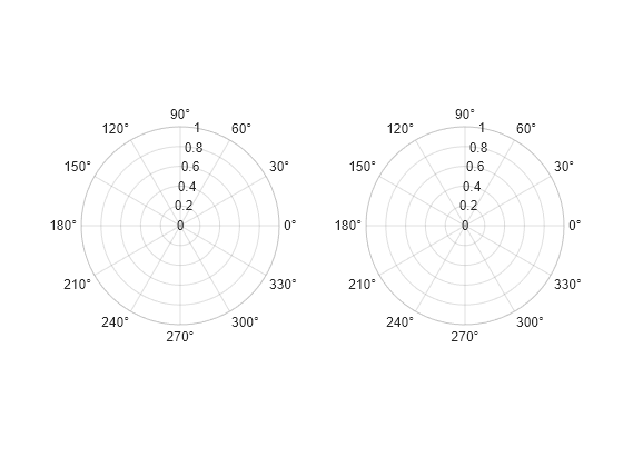
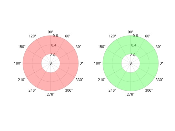
Create a red radius region in the first polar axes, and create a green radius region in the second polar axes. Specify the PolarAxes object that you want to plot into as the first argument when you call radiusregion.
r1 = 0.2;
r2 = 0.6;
radiusregion(pax1,r1,r2,FaceColor="r")
radiusregion(pax2,r1,r2,FaceColor="g")
Input Arguments
Inner and outer radii, specified as a pair of scalars or a pair of vectors. To
create one filled region, specify r1 and r2 as
scalars. To create multiple filled regions, specify vectors of equal length. You can
specify the radius values in any order. Thus, radiusregion(1,5) and
radiusregion(5,1) produce the same result.
To create an unbounded region, specify one of the radii as
Inf. Specifying a value of –Inf creates a filled
circle centered at r=0.
If any radii are NaN values, no region appears for those
radii.
Example: radiusregion(0.5,1) creates a filled region from
r=0.5 to r=1.
Example: radiusregion([1 3],[2 4]) creates two filled regions: one
from r=1 to r=2 and the other from
r=3 to r=4.
Data Types: single | double
Inner and outer radii for multiple regions, specified as a 2-by-n or n-by-2 matrix, where n is the number of regions. If you specify a 2-by-2 matrix, each column of the matrix corresponds to a region.
To create an unbounded region, specify one of the radii as
Inf. Specifying a value of –Inf creates a filled
circle centered at r=0.
If any radii are NaN values, no region appears for those
radii.
Example: radiusregion([1 3; 2 4]) creates a filled region from
r=1 to r=2, and another filled region from
r=3 to r=4.
Data Types: single | double
Target polar axes for the filled region, specified as a PolarAxes
object. Use this argument if you want to create the filled region in a specific
PolarAxes object instead of the current axes.
Name-Value Arguments
Specify optional pairs of arguments as
Name1=Value1,...,NameN=ValueN, where Name is
the argument name and Value is the corresponding value.
Name-value arguments must appear after other arguments, but the order of the
pairs does not matter.
Example: radiusregion(0.5,1,FaceColor="yellow") creates a yellow
filled region.
Note
The properties listed here are only a subset. For a complete list, see PolarRegion Properties.
Fill color, specified as an RGB triplet, a hexadecimal color code, or a color name.
For a custom color, specify an RGB triplet or a hexadecimal color code.
An RGB triplet is a three-element row vector whose elements specify the intensities of the red, green, and blue components of the color. The intensities must be in the range
[0,1], for example,[0.4 0.6 0.7].A hexadecimal color code is a string scalar or character vector that starts with a hash symbol (
#) followed by three or six hexadecimal digits, which can range from0toF. The values are not case sensitive. Therefore, the color codes"#FF8800","#ff8800","#F80", and"#f80"are equivalent.
Alternatively, you can specify some common colors by name. This table lists the named color options, the equivalent RGB triplets, and the hexadecimal color codes.
| Color Name | Short Name | RGB Triplet | Hexadecimal Color Code | Appearance |
|---|---|---|---|---|
"red" | "r" | [1 0 0] | "#FF0000" |
|
"green" | "g" | [0 1 0] | "#00FF00" |
|
"blue" | "b" | [0 0 1] | "#0000FF" |
|
"cyan"
| "c" | [0 1 1] | "#00FFFF" |
|
"magenta" | "m" | [1 0 1] | "#FF00FF" |
|
"yellow" | "y" | [1 1 0] | "#FFFF00" |
|
"black" | "k" | [0 0 0] | "#000000" |
|
"white" | "w" | [1 1 1] | "#FFFFFF" |
|
"none" | Not applicable | Not applicable | Not applicable | No color |
This table lists the default color palettes for plots in the light and dark themes.
| Palette | Palette Colors |
|---|---|
Before R2025a: Most plots use these colors by default. |
|
|
|
You can get the RGB triplets and hexadecimal color codes for these palettes using the orderedcolors and rgb2hex functions. For example, get the RGB triplets for the "gem" palette and convert them to hexadecimal color codes.
RGB = orderedcolors("gem");
H = rgb2hex(RGB);
Before R2023b: Get the RGB triplets using RGB =
get(groot,"FactoryAxesColorOrder").
Before R2024a: Get the hexadecimal color codes using H =
compose("#%02X%02X%02X",round(RGB*255)).
Boundary line color, specified as an RGB triplet, a hexadecimal color code, or a color name.
For a custom color, specify an RGB triplet or a hexadecimal color code.
An RGB triplet is a three-element row vector whose elements specify the intensities of the red, green, and blue components of the color. The intensities must be in the range
[0,1], for example,[0.4 0.6 0.7].A hexadecimal color code is a string scalar or character vector that starts with a hash symbol (
#) followed by three or six hexadecimal digits, which can range from0toF. The values are not case sensitive. Therefore, the color codes"#FF8800","#ff8800","#F80", and"#f80"are equivalent.
Alternatively, you can specify some common colors by name. This table lists the named color options, the equivalent RGB triplets, and the hexadecimal color codes.
| Color Name | Short Name | RGB Triplet | Hexadecimal Color Code | Appearance |
|---|---|---|---|---|
"red" | "r" | [1 0 0] | "#FF0000" |
|
"green" | "g" | [0 1 0] | "#00FF00" |
|
"blue" | "b" | [0 0 1] | "#0000FF" |
|
"cyan"
| "c" | [0 1 1] | "#00FFFF" |
|
"magenta" | "m" | [1 0 1] | "#FF00FF" |
|
"yellow" | "y" | [1 1 0] | "#FFFF00" |
|
"black" | "k" | [0 0 0] | "#000000" |
|
"white" | "w" | [1 1 1] | "#FFFFFF" |
|
"none" | Not applicable | Not applicable | Not applicable | No color |
This table lists the default color palettes for plots in the light and dark themes.
| Palette | Palette Colors |
|---|---|
Before R2025a: Most plots use these colors by default. |
|
|
|
You can get the RGB triplets and hexadecimal color codes for these palettes using the orderedcolors and rgb2hex functions. For example, get the RGB triplets for the "gem" palette and convert them to hexadecimal color codes.
RGB = orderedcolors("gem");
H = rgb2hex(RGB);
Before R2023b: Get the RGB triplets using RGB =
get(groot,"FactoryAxesColorOrder").
Before R2024a: Get the hexadecimal color codes using H =
compose("#%02X%02X%02X",round(RGB*255)).
Fill color transparency, specified as a scalar in the range [0,1]. A value of 1 is opaque and 0 is completely transparent. Values between 0 and 1 are partially transparent.
Boundary line style, specified as one of the options listed in this table.
| Line Style | Description | Resulting Line |
|---|---|---|
"-" | Solid line |
|
"--" | Dashed line |
|
":" | Dotted line |
|
"-." | Dash-dotted line |
|
"none" | No line | No line |
Version History
Introduced in R2024a
MATLAB Command
You clicked a link that corresponds to this MATLAB command:
Run the command by entering it in the MATLAB Command Window. Web browsers do not support MATLAB commands.
Web サイトの選択
Web サイトを選択すると、翻訳されたコンテンツにアクセスし、地域のイベントやサービスを確認できます。現在の位置情報に基づき、次のサイトの選択を推奨します:
また、以下のリストから Web サイトを選択することもできます。
最適なサイトパフォーマンスの取得方法
中国のサイト (中国語または英語) を選択することで、最適なサイトパフォーマンスが得られます。その他の国の MathWorks のサイトは、お客様の地域からのアクセスが最適化されていません。
南北アメリカ
- América Latina (Español)
- Canada (English)
- United States (English)
ヨーロッパ
- Belgium (English)
- Denmark (English)
- Deutschland (Deutsch)
- España (Español)
- Finland (English)
- France (Français)
- Ireland (English)
- Italia (Italiano)
- Luxembourg (English)
- Netherlands (English)
- Norway (English)
- Österreich (Deutsch)
- Portugal (English)
- Sweden (English)
- Switzerland
- United Kingdom (English)