Create Maps with Data in Projected Coordinate Reference Systems

Example 1: Import Raster Data in Projected Coordinate Reference System

Geographic raster data that contains coordinates in a projected coordinate reference system can be stored in a variety of different formats, including standard file formats such as GeoTIFF, Spatial Data Transfer Standard (SDTS), NetCDF, HDF4, or HDF5. This example illustrates importing data from a GeoTIFF file. The data in the file contains coordinates in the projected map coordinate reference system Massachusetts State Plane Mainland Zone coordinate system.

The coordinates of the image in the GeoTIFF file, boston.tif, are in a projected coordinate reference system. You can determine that by using the geotiffinfo function and examine the PCS and Projection field values.

info = geotiffinfo('boston.tif');
disp(info.PCS)

NAD83 / Massachusetts Mainland

disp(info.Projection)

SPCS83 Massachusetts Mainland zone (meter)

The length unit of the coordinates are defined by the UOMLength field in the info structure.

disp(info.UOMLength)

US survey foot

To import the image and the spatial referencing object, use readgeoraster.

[boston,R] = readgeoraster('boston.tif');

Example 2: Display Raster Data in Projected Coordinate Reference System

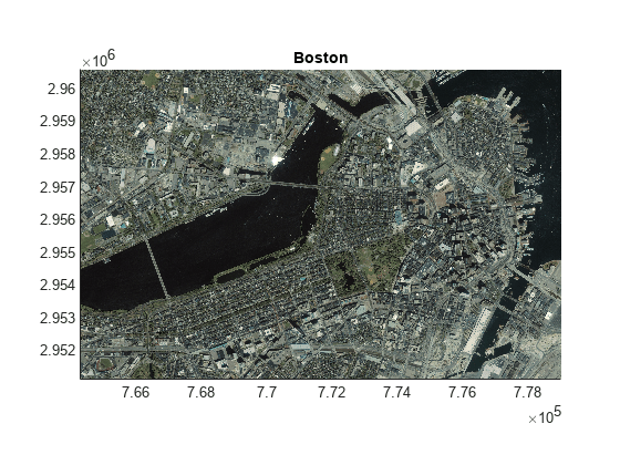
You can display the image on a regular MATLAB axes using mapshow, which displays the image and sets the axes limits to the limits defined by the referencing object, R. The coordinates, as mentioned above, are in US survey foot and are relative to an origin to the southwest of the map, which is why the numbers are large. The coordinates are always positive within the zone.

mapshow(boston,R)
axis image
title('Boston')

Example 3: Import Vector Data in Projected Coordinate Reference System

Geographic vector data that contains coordinates in a projected coordinate reference system can be stored in shapefiles. This example illustrates how to import vector data in a projected coordinate reference system from the shapefile, boston_roads.shp.

Import vector line data from the boston_roads.shp file as a geospatial table.

roads = readgeotable('boston_roads.shp');

The Shape variable of the table contains information about the line shapes. Query the projected coordinate reference system of the shapes.

roads.Shape.ProjectedCRS

ans = 
  projcrs with properties:

                    Name: "NAD83 / Massachusetts Mainland"
           GeographicCRS: [1×1 geocrs]
        ProjectionMethod: "Lambert Conic Conformal (2SP)"
              LengthUnit: "meter"
    ProjectionParameters: [1×1 map.crs.ProjectionParameters]

Example 4: Display Vector and Raster Data in Projected Coordinate Reference System

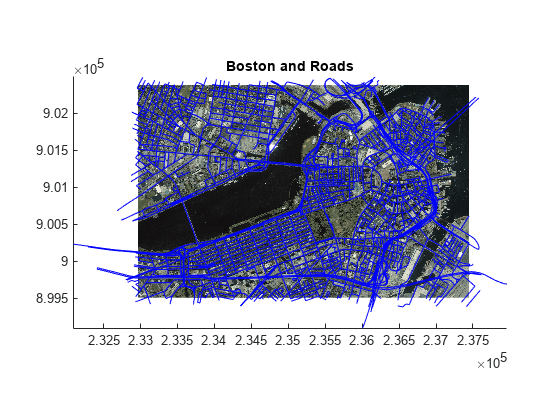
The vector and raster data in this example are in the same projected coordinate reference system. However, the vector data is in length units of meter, while the raster data is in length unit of survey foot. Convert the raster data to length units of meter and display the data on the same axes.

Convert the coordinates of the raster image from units of US survey foot to meter.

R.XWorldLimits = R.XWorldLimits * unitsratio('m','sf');
R.YWorldLimits = R.YWorldLimits * unitsratio('m','sf');

Display the raster image and vector data using mapshow.

figure
mapshow(boston,R)
mapshow(roads)
title('Boston and Roads')

Example 5: Display Data in both Geographic and Projected Coordinate Reference Systems

You may have geographic data whose coordinates are in latitude and longitude and other data whose coordinates are in a projected coordinate reference system. You can display these data sets in the same map display. This example illustrates how to display data in a geographic coordinate reference system (latitude and longitude) with data in a projected map coordinate reference system (Massachusetts State Plane Mainland Zone coordinate system).

Read a raster image with a worldfile whose coordinates are in latitude and longitude. Use imread to read the image and worldfileread to read the worldfile and construct a spatial referencing object.

filename = 'boston_ovr.jpg';
overview = imread(filename);
overviewR = worldfileread(getworldfilename(filename), 'geographic', size(overview));

To display the overview image and the GeoTIFF image in the same map display, you need to create a map display using a Mapping Toolbox™ projection structure containing the projection information for the data in the projected coordinate reference system, Massachusetts State Plane Mainland Zone coordinate system. To make a map display in this system, you can use the projection information contained in the GeoTIFF file. Use the geotiff2mstruct function to construct a Mapping Toolbox™ projection structure, from the contents of the GeoTIFF information structure. The geotiff2mstruct function returns a projection in units of meters. Use the projection structure to define the projection parameters for the map display.

mstruct = geotiff2mstruct(info);

Use the latitude and longitude limits of the Boston overview image.

latlim = overviewR.LatitudeLimits;
lonlim = overviewR.LongitudeLimits;

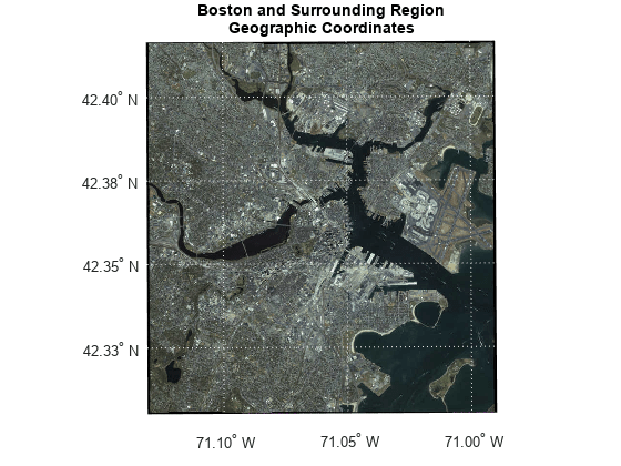
Create an axesm-based map by using the projection information stored in the map projection structure and set the map latitude and longitude limits. Display the geographic data in the map. geoshow projects the latitude and longitude coordinates.

figure
ax = axesm(mstruct, 'Grid', 'on',...
    'GColor', [.9 .9 .9], ...
    'MapLatlimit', latlim, 'MapLonLimit', lonlim, ...
    'ParallelLabel', 'on', 'PLabelLocation', .025, 'PlabelMeridian', 'west', ...
    'MeridianLabel', 'on', 'MlabelLocation', .05, 'MLabelParallel', 'south', ...
    'MLabelRound', -2, 'PLabelRound', -2, ...
    'PLineVisible', 'on', 'PLineLocation', .025, ...
    'MLineVisible', 'on', 'MlineLocation', .05);
geoshow(overview, overviewR)
axis off
tightmap
title({'Boston and Surrounding Region', 'Geographic Coordinates'})

Since the coordinates of the GeoTIFF image are in a projected coordinate reference system, use mapshow to overlay the more detailed Boston image onto the display. Plot the boundaries of the Boston image in red.

mapshow(boston, R)
plot(R.XWorldLimits([1 1 2 2 1]), R.YWorldLimits([1 2 2 1 1]), 'Color', 'red')
title({'Boston and Surrounding Region', 'Geographic and Projected Coordinates'})

Zoom to the geographic region of the GeoTIFF image by setting the axes limits to the limits of the Boston image and add a small buffer. Note that the buffer size (delta) is expressed in meters.

delta = 1000;
xLimits = R.XWorldLimits + [-delta delta];
yLimits = R.YWorldLimits + [-delta delta];
xlim(ax,xLimits)
ylim(ax,yLimits)
setm(ax, 'Grid', 'off');

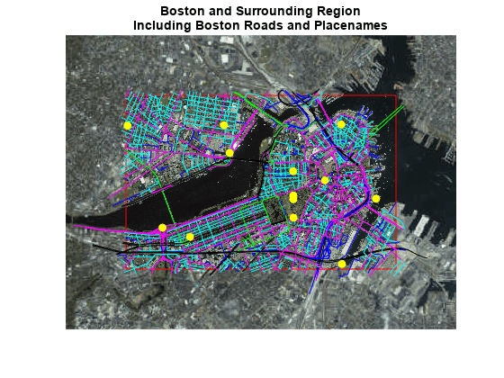
You can overlay the road vectors onto the map display. Use a symbol specification to give each class of road its own color.

roadColors = makesymbolspec('Line',...
    {'CLASS', 2, 'Color', 'k'}, ...
    {'CLASS', 3, 'Color', 'g'},...
    {'CLASS', 4, 'Color', 'magenta'}, ...
    {'CLASS', 5, 'Color', 'cyan'}, ...
    {'CLASS', 6, 'Color', 'b'},...
    {'Default',  'Color', 'k'});
mapshow(roads, 'SymbolSpec', roadColors)
title({'Boston and Surrounding Region','Including Boston Roads'})

You can also overlay data from a GPS stored in a GPX file. Import point geographic vector data from the boston_placenames.gpx file included with the Mapping Toolbox™ software. The file contains latitude and longitude coordinates of geographic point features in part of Boston, Massachusetts, USA.

places = readgeotable('boston_placenames.gpx');

Overlay the places onto the map and increase the marker size, change the markers to circles and set their edge and face colors to yellow.

geoshow(places, 'Marker','o', 'MarkerSize', 6, ...
    'MarkerEdgeColor', 'y', 'MarkerFaceColor','y')
title({'Boston and Surrounding Region','Including Boston Roads and Placenames'})

Data Set Information

The files boston.tif and boston_ovr.jpg include materials copyrighted by GeoEye, all rights reserved. GeoEye was merged into the DigitalGlobe corporation on January 29th, 2013. For more information about the data sets, use the commands type boston.txt and type boston_ovr.txt.

The files boston_roads.shp and boston_placenames.gpx are from the Bureau of Geographic Information (MassGIS), Commonwealth of Massachusetts, Executive Office of Technology and Security Services. For more information about the data sets, use the commands type boston_roads.txt and type boston_placenames_gpx.txt.