Perform Sensitivity and Yield Analysis of Optical Coating Using Monte Carlo

This example demonstrates how to calculate the sensitivity of optical coating layers in a Bragg reflector. To estimate the expected manufacturing yield, you then implement Monte Carlo simulation that incorporates material-specific tolerances in layer thickness and refractive index. Monte Carlo (MC) simulation is a statistical method that estimates system performance by repeatedly evaluating the design with randomized variations in its parameters. Each MC trial represents one possible manufactured coating, created by sampling all layer thicknesses and refractive indices according to their specified tolerances. This approach quantifies how sensitive the coating’s optical performance is to real-world process variations, and predicts the proportion of manufactured parts, or the yield, expected to meet the required specifications.

Specify Design Parameters

First, specify the range of design angles of incidence, in degrees, and the range of wavelengths, in nanometers.

design.Angles = 0:5:15;
design.Wavelengths = 512:552;

Specify the minimum average reflectivity required for the selected design angles and wavelengths. This value can range from 0.90 to over 0.99 depending on the application and cost. To achieve a higher average reflectivity, you must to use more layers, at the expense of higher manufacturing costs.

design.RMinReq = 0.940;

Create Bragg Optical Coating

A Bragg reflector uses alternating layers of high and low index of refraction materials to achieve reflection by constructive interference of light. In this example, you create a Bragg reflector that consists of alternating TiO2 and SiO2 layers, which have a high and low index of refraction, respectively.

Create a 10-layer Bragg reflector at 532 nm with a Quarter Wavelength Optical Thickness (QWOT) using the opticalCoating object. The first TiO2 layer is adjacent to the substrate and last layer, SiO2, is exposed to the medium. Specify the units of thickness as the quarter wavelength using the ThicknessUnit name-value argument.

numLayers = 10;
oc = opticalCoating(...
    Name= "Bragg Reflector 532nm", ...
    CoatingMaterials = ["TiO2","SiO2"], ...
    WavelengthRange = [min(design.Wavelengths) max(design.Wavelengths)], ...
    IncidentAngleRange = [min(design.Angles) max(design.Angles)], ...
    PrimaryWavelength = 532, ...
    LayerMaterialIndex = repmat([1 2], [1 numLayers/2]), ...
    ThicknessUnit="quarterWavelength", ...
    LayerThickness=ones(1,numLayers));

After you create the optical coating, change the thickness units to nanometers for layer thickness manipulations. Changing the units does not affect the actual physical thickness, but only updates the LayerThickness property to display and accept values in your selected units.

oc.ThicknessUnit = "nm";

Visualize Nominal Reflectivity Performance

Select a wider wavelength band to visualize the reflectivity response.

dispWavelength = 400:700;

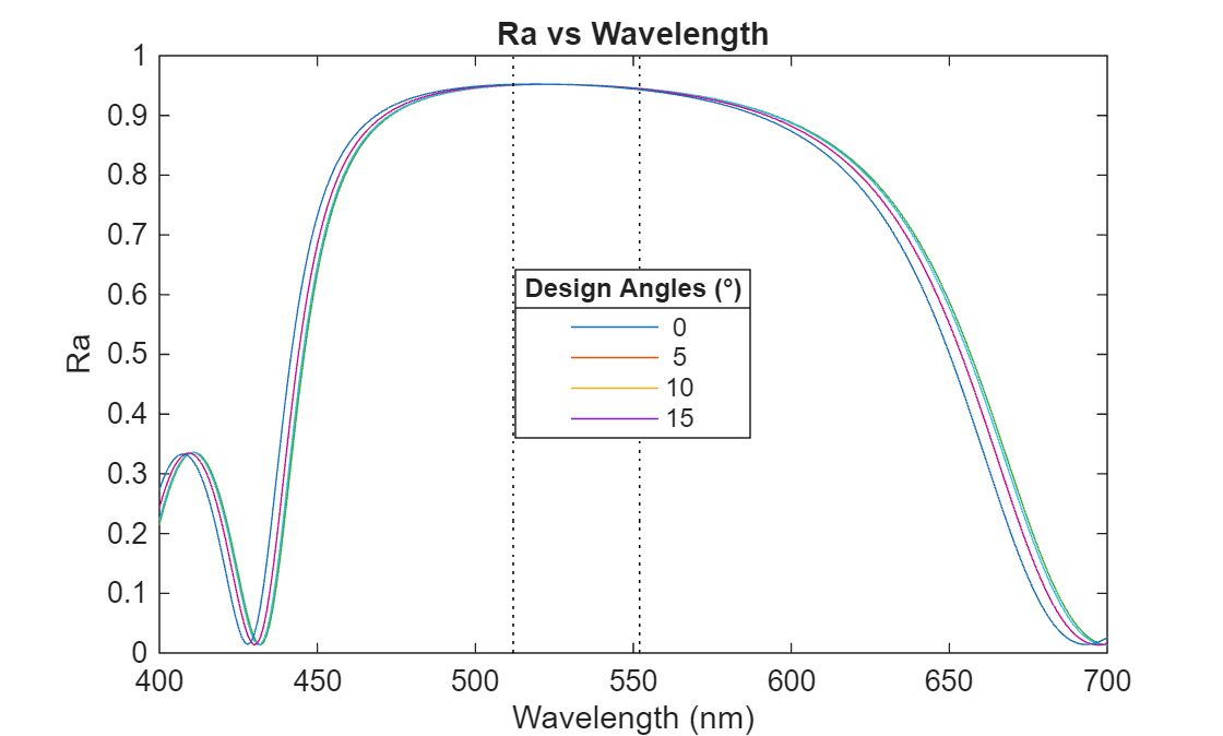
Compute the average reflectivity, Ra, across the range of design wavelengths and angles. Observe the shift in reflectivity toward shorter wavelengths at higher incident angles, a phenomenon known as "blue-shift" that results from the increased effective refractive index at oblique incidence.

fq = fresnelCoefficients(oc, ...
    Wavelengths=dispWavelength,IncidentAngles=design.Angles);
plot(dispWavelength,fq.Ra');
hold on;
plot([oc.WavelengthRange(1),oc.WavelengthRange(1)],[0 1],"k:");
plot([oc.WavelengthRange(2),oc.WavelengthRange(2)],[0 1],"k:");
title("Ra vs Wavelength")
l1 = legend(num2str(design.Angles'),Location="best");
xlabel("Wavelength (nm)");
ylabel("Ra");
title(l1,"Design Angles (°)")

Perform Sensitivity Analysis

Define a merit function to evaluate coating performance for a given sample. This function returns the minimum average reflectivity, Ra, within the reflection band and a pass/fail flag based on the design requirement. First, compute the minimum Ra in the reflection band as a performance metric. Then, set the pass/fail criterion according to the specified design requirement.

function [rmin,pf] = coatingMerit(oc,design)
fq = fresnelCoefficients(oc, ...
    Wavelengths=design.Wavelengths,IncidentAngles=design.Angles);
rmin = min(fq.Ra(:));
pf = rmin>=design.RMinReq;
end

Compute the nominal minimum reflectivity for the design.

RMinNominal = coatingMerit(oc,design);

To estimate layer sensitivity, vary each layer thickness within a fixed range (+/- 2 nm). For each layer, compute the maximum reduction in Ra relative to the nominal design.

thicknessTol = 2;
layerSensitivity = zeros(1,oc.NumLayers);
for lInd = 1:oc.NumLayers
    ocSensitivity = oc;
    nomThickness = oc.LayerThickness(lInd);

    % Compute response for the lower bound
    ocSensitivity.LayerThickness(lInd) = nomThickness-thicknessTol;
    RMin = coatingMerit(ocSensitivity, design);
    minThickSensitivity = max(0,RMinNominal-RMin);

    % Compute response for the upper bound
    ocSensitivity.LayerThickness(lInd) = nomThickness+thicknessTol;
    RMin = coatingMerit(ocSensitivity, design);
    maxThickSensitivity = max(0,RMinNominal-RMin);

    layerSensitivity(lInd) = max(minThickSensitivity, maxThickSensitivity);
end

Visualize the sensitivity of each layer.

figure
bar(1:oc.NumLayers,layerSensitivity,FaceAlpha=0.3)
xlabel("Layer Number")
ylabel("Max Dip in Ra Relative to Nominal")
title("Layer Sensitivity Analysis")

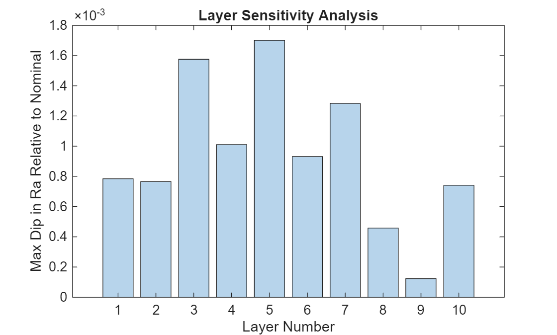
This plot indicates that the middle layers exhibit greater sensitivity to thickness variations compared to the outer layers, highlighting the need for more precise control and tighter tolerances for these layers during fabrication.

This approach provides a quick estimate of layer sensitivity using fixed thickness perturbations. A more detailed, material-specific analysis is performed in the subsequent Monte Carlo section.

Monte Carlo Tolerance Analysis and Yield Estimation

Using Monte Carlo analysis, you will simulate a large number of manufacturing runs by randomly varying each sample's layer thicknesses and refractive indices within specified process limits. By evaluating the optical performance of each simulated coating, you estimate the manufacturing yield as the percentage of samples that meet the design specifications.

Start with a smaller number of trials for visualization. Increase numTrials for more accurate yield estimates, such as 5,000 or more, or until results converge.

numTrials  = 400;
showGraphs = numTrials<600;

Specify standard deviations for thickness and refractive index variations, based on material and process capability. The order of the thickness and index of refraction variations should match the coating materials in the CoatingMaterials property of oc.

thicknessSigma = [2 1.5];
NdSigma = [0.008 0.004];

Clear previous simulation data.

clear MCTrial

Run the Monte Carlo simulation in parallel, perturbing all layer thicknesses and material indices independently for each trial. To run the simulation in parallel, you need a Parallel Computing Toolbox™ license. For more information, see Use parfor to Speed Up Monte-Carlo Code (Parallel Computing Toolbox).

tic
parfor tInd = 1:numTrials

    % Perturb refractive index for each material.
    cm = opticalMaterial.empty();
    for cmInd = numel(oc.CoatingMaterials):-1:1
        % Look-up table of [Nd, Wavelength]
        ndLut = oc.CoatingMaterials(cmInd).RefractiveIndexParameter;
        % Perturb Nd values 
        ndLut(:,1) = ndLut(:,1) ...
            + randn(size(ndLut(:,1))) * NdSigma(cmInd);
        % Create perturbed material sample to use for this trial
        cm(cmInd) = opticalMaterial(...
            RefractiveIndexMethod = "LookupTable", ...
            RefractiveIndexParameter = ndLut, ...
            TransmissionParameters=oc.CoatingMaterials(cmInd).TransmissionParameters);
    end

    % Perturb all layer thicknesses independently.
    perturbedThickness = oc.LayerThickness...
        + randn(size(oc.LayerThickness)) .* thicknessSigma(oc.LayerMaterialIndex);

    % Create a sample for this trial using perturbed thickness and
    % indexes of refraction.
    ocMC = opticalCoating(CoatingMaterials=cm, ...
        WavelengthRange=oc.WavelengthRange, ...
        IncidentAngleRange=oc.IncidentAngleRange, ...
        PrimaryWavelength=oc.PrimaryWavelength, ...
        LayerMaterialIndex=oc.LayerMaterialIndex, ...
        ThicknessUnit=oc.ThicknessUnit, ...
        LayerThickness=perturbedThickness);

    if showGraphs
        % Store reflectivity for visualization.
        fq = fresnelCoefficients(ocMC, ...
            Wavelengths=dispWavelength,IncidentAngles=design.Angles);
        MCTrial(tInd).Ra = fq.Ra;
    end

    % Evaluate performance and pass/fail status
    [~,MCTrial(tInd).Pass] = coatingMerit(ocMC,design);

end
toc

Elapsed time is 19.597465 seconds.

Compute and display the yield.

numPassSamples = sum([MCTrial.Pass]);
yieldPercent = numPassSamples/numTrials*100;
disp("Yield is: "+yieldPercent+"%");

Yield is: 80.5%

if ~showGraphs
    return
end

Note: This MC analysis incorporates material-dependent process tolerances. For large numbers of trials, visualization is disabled to improve performance.

Visualize Monte Carlo Reflectivity Envelopes

Aggregate the Monte Carlo simulation results to compute the minimum and maximum reflectivity Ra envelopes across all samples. Compare the nominal response to the MC tolerance envelope for each angle of incidence.

fq = fresnelCoefficients(oc,...
    Wavelengths=dispWavelength, IncidentAngles=design.Angles);
nominalRa = fq.Ra;
minEnvelope = inf(size(nominalRa));
maxEnvelope = zeros(size(nominalRa));

for tInd = 1:numTrials
    minEnvelope = min(minEnvelope, MCTrial(tInd).Ra);
    maxEnvelope = max(maxEnvelope, MCTrial(tInd).Ra);
end

Plot the nominal response and the MC envelope for each incident angle. The nominal Ra is shown as a green line. The tolerance envelope is shaded in yellow. The required minimum Ra is indicated by a red line, the reflection band by black lines, and the primary wavelength by a blue line.

figure
numAngles = numel(design.Angles);
tiledlayout("flow");
hax = gobjects(1, numAngles);

for aInd = 1:numAngles

hax(aInd) = nexttile;

    % Nominal Ra (green)
    plot(dispWavelength,nominalRa(aInd,:),"g-",LineWidth=2)
    hold on

    % Required Ra minimum (red)
    [lw, uw] = bounds(dispWavelength);
    lTol = design.RMinReq;
    plot([lw uw], [lTol lTol],"r");

    % Reflection band (black)
    plot([oc.WavelengthRange(1),oc.WavelengthRange(1)],[0 1],"k");
    plot([oc.WavelengthRange(2),oc.WavelengthRange(2)],[0 1],"k");

    % Primary wavelength (blue)
    plot([oc.PrimaryWavelength,oc.PrimaryWavelength],[0 1],"b");

    % Tolerance envelope (yellow)
    fill([dispWavelength fliplr(dispWavelength)], ...
        [maxEnvelope(aInd,:) fliplr(minEnvelope(aInd,:))], ...
        "r",FaceAlpha=0.2,EdgeColor="none")

    xlabel("Wavelength (nm)")
    ylabel("Reflection")

    title(design.Angles(aInd) + "°");
    grid on
end

% Shared legend
hl = legend("Nominal","Min Required Ra","","","Tolerance Envelope");
hl.Layout.Tile = numAngles + 1;

% Link axes for interactive zoom
linkaxes(hax)

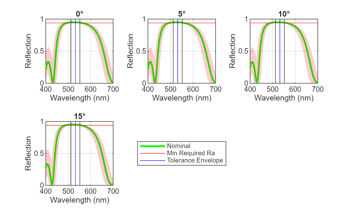
This visualization highlights the effect of process variation on reflectivity. The tolerance envelope shows the range of possible Ra values due to manufacturing variability, allowing easy comparison to design requirements.

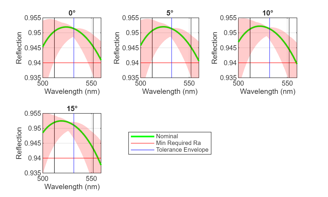
For a more detailed view of how the reflectivity varies within the critical wavelength range specified for the coating's performance, zoom in on the reflection band.

xlim([500 560])
ylim([0.935 0.955])

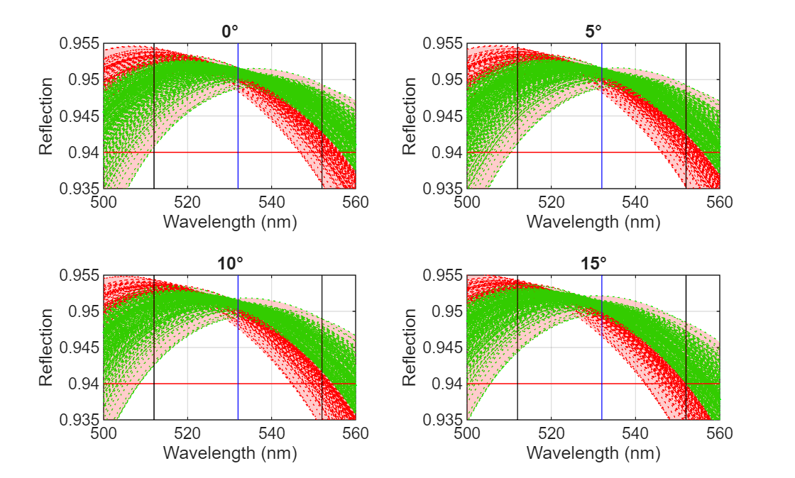
Visualize Individual Monte Carlo Trial Responses

Inspect individual MC trial reflectivity responses for sanity checking with a small number of samples. Each trial is plotted as a dotted line: green for passing samples, red for failing samples. A sample is considered failing if Ra drops below the required minimum at any angle, so a red line in any plot means that sample failed at least one angle.

for aInd = 1:numAngles
axes(hax(aInd));
    legend off
    
    % Prepare data with NaN separators for efficient plotting
    passingX = []; passingY = []; failingX = []; failingY = [];    
    for tInd = 1:numTrials
        if MCTrial(tInd).Pass
            passingX = [passingX, dispWavelength, NaN];
            passingY = [passingY, MCTrial(tInd).Ra(aInd,:), NaN];
        else
            failingX = [failingX, dispWavelength, NaN];
            failingY = [failingY, MCTrial(tInd).Ra(aInd,:), NaN];
        end
    end
    
    % Plot passing trials (green dotted)
    if ~isempty(passingY)
        h = plot(passingX,passingY,"g:");
        uistack(h,"bottom");
    end
    
    % % Plot failing trials (red dotted)
    if ~isempty(failingY)
        h = plot(failingX, failingY,"r:");
        uistack(h,"bottom");
    end
end