mtf
R2026bDescription
Add-On Required: This feature requires the Optical Design and Simulation Library for Image Processing Toolbox add-on.
mtfr = mtf(opsys)opsys using the default field points and wavelengths. The MTF
represents contrast transfer as a function of spatial frequency in the image plane. The
function computes MTF from a PSF generated for the specified field points and
wavelengths.
mtfr = mtf(opsys,Name=Value)mtf(opsys,FieldPoints=fp,Wavelengths=587.56,Method="Huygens")
computes a wave-optics MTF for the field point fp at a wavelength of
587.56 nanometers. The function uses these options to generate the PSF from which it
computes the MTF.
Examples
Load the sample Double Gauss lens system using zmximport. Define an off-axis field point at an angle of 3 degrees along the y-axis, and compute the geometric MTF for three distinct wavelengths (486.1 nm, 587.6 nm, and 656.3 nm).
opsys = zmximport("DoubleGaussLens.zmx");
fp = fieldPoint(Angles=[0 3]);
mtfr = mtf(opsys, FieldPoints=fp, Wavelengths=[486.1 587.6 656.3])
mtfr =
GeometricMTF with properties:
Tangential: [1×1 struct]
Sagittal: [1×1 struct]
FieldPoint: [1×1 optics.fieldpoint.FieldAngle]
Wavelengths: [486.1000 587.6000 656.3000]
FFTLength: [128 128]
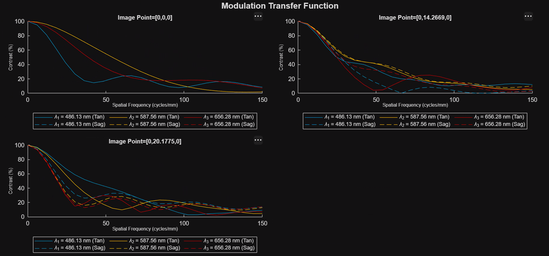
Load the sample Double Gauss lens system using zmximport. Compute the Huygens MTF by setting the Method name-value argument to "Huygens". Limit the output curves to a spatial frequency of 150 cycles per millimeter using the MaximumFrequency argument, and specify an FFTLength of 512 to achieve higher frequency resolution.
opsys = zmximport("DoubleGaussLens.zmx");
mtfr = mtf(opsys, Method="Huygens", MaximumFrequency=150, FFTLength=512);
Visualize the tangential and sagittal contrast curves as a function of spatial frequency by passing the result object to the show function.
hmtf = show(mtfr)
hmtf =
  MTFChart with properties:

               Legend: on
                 Grid: "off"
                Title: "Modulation Transfer Function"
                  MTF: [1×3 optics.result.HuygensMTF]
    WavelengthIndices: [1 2 3]
                Color: [3×3 double]
             Position: [0.0737 0.2521 0.8713 0.5977]
                Units: 'normalized'

  Show all properties
Load the sample Double Gauss lens system using zmximport. Compute the geometric MTF up to a maximum spatial frequency of 200 cycles per millimeter by setting the MaximumFrequency name-value argument.
opsys = zmximport("DoubleGaussLens.zmx");
mtfr = mtf(opsys, MaximumFrequency=200);
Use the frequencyAtContrast function to compute MTF50, the spatial frequency where the MTF first drops to 50% contrast. Then, use the contrastAtFrequency function to determine the exact sagittal and tangential contrast values at spatial frequencies of 30, 60, and 100 cycles per millimeter.
By default, these functions evaluate the entire optical system simultaneously and return multi-dimensional arrays. The dimensions map to [Fields, Wavelengths, Configurations, Planes] for the MTF50 output, and [Fields, Wavelengths, Frequencies, Planes] for the contrast output, where the rows represent field points and the columns represent wavelengths.
MTF50 = frequencyAtContrast(mtfr, 0.5)
MTF50 =
MTF50(:,:,1,1) =

   22.2302   48.5808   37.1994
   30.4516   44.1749   35.1107
   26.2930   20.7316   19.6589


MTF50(:,:,1,2) =

   22.2300   48.5906   37.2039
   31.2080   43.8519   27.4440
   52.5096   33.6761   18.1949
contrast = contrastAtFrequency(mtfr, [30; 60; 100])
contrast =
contrast(:,:,1,1) =

    0.4014    0.7605    0.6261
    0.5084    0.6298    0.5519
    0.4752    0.3834    0.3539


contrast(:,:,2,1) =

    0.2572    0.3637    0.2569
    0.1174    0.3793    0.2909
    0.3216    0.2569    0.2353


contrast(:,:,3,1) =

    0.1793    0.0742    0.2620
    0.0475    0.1648    0.0820
    0.2108    0.1898    0.1699


contrast(:,:,1,2) =

    0.4014    0.7606    0.6262
    0.5081    0.6205    0.4417
    0.7480    0.5750    0.3493


contrast(:,:,2,2) =

    0.2572    0.3639    0.2569
    0.2959    0.3558    0.1313
    0.4327    0.2412    0.2650


contrast(:,:,3,2) =

    0.1793    0.0742    0.2618
    0.0944    0.1362    0.1943
    0.0866    0.2809    0.2394
Input Arguments
Name-Value Arguments
Output Arguments
More About
Version History
Introduced in R2026b
See Also
psf | airyDiskRadius | GeometricMTF | HuygensMTF | contrastAtFrequency | frequencyAtContrast | spot | opticalSystem | fieldPoint | MTFChart

