Optimize Coating Design for Longpass Optical Filter

This example demonstrates how to design a 550 nm longpass optical filter, accounting for material properties and manufacturing limits using the Optimization Explorer (Optimization Toolbox) app. The method can be extended to more complex multi-band filters.

Specify Optical Filter Design Manufacturing Constraints

Begin by specifying the filter design parameters, including materials, allowable thickness ranges, layer count, and spectral requirements.

First, specify the filter name and the required reference wavelength, in nanometers. Since the various stop and pass bands are explicitly specified later, the primary wavelength is not explicitly used in the design process. Specifying any wavelength within the band ranges is sufficient.

design.Name = "550nm Longpass";
design.PrimaryWavelength = 550;

Define the coating materials, the two most common low and high index of refraction materials, SiO₂ and TiO2.

design.Materials = [pickCoatingMaterial("SiO2"), ...
    pickCoatingMaterial("TiO2")];
disp([design.Materials.Nd])

    1.4586    2.3247

Specify N-BK7 glass as the substrate material.

design.Substrate = pickGlass("N-BK7");

Specify the number of total layers. Use an even number of layers for a stack of alternating high and low refractive index layers. However, this can be relaxed in conjunction with how the LayerMaterialIndex and bounds are specified later. Increase the number of layers to help achieve stringent stop band, edge width, and pass band ripple constraints at the expense of manufacturing costs.

design.NumberOfLayers = 48; 

Set SiO₂ (material index 2) as the first layer to ensure good adhesion to the substrate, and alternate between SiO₂ and TiO₂ for the remaining layers. Use SiO₂ as the top layer for durability. To use different materials or a custom sequence, modify the LayerMaterialIndex array. If consecutive layers use the same material, combine them and ensure the total thickness stays within manufacturing limits.

design.LayerMaterialIndex = repmat([2 1],[1 design.NumberOfLayers/2]);

Specify the minimum and maximum layer thicknesses for each material, in nanometers.

design.MinLayerThickness = [20 20]; 
design.MaxLayerThickness = [50 150];

Specify the range of wavelengths, in nanometers, and angles, in degrees, for which to visualize the coatings response.

design.WavelengthRange = [350 750];
design.AngleRange = [0 10];

Specify Optical Response Requirements

In this section, you define the desired optical performance using a goals structure. For a longpass filter, you must configure both stop band and pass band requirements.

First, specify the stop band. The stop band blocks wavelengths below the cut-on frequency. Set the minimum required optical density (OD) in this region. OD is calculated as -log₁₀(Ta), where Ta is the total transmission. For most applications, OD ≥ 2 (Ta < 0.01) is a typical minimum. Define the stop band wavelength range as 350 - 545 nm, the angles of incidence as 0 and 5 degrees, and assign a weight to this band in the merit function. Higher weights make the optimizer prioritize meeting these requirements.

goals.ODCutOff = 2;
goals.Bands(1).ResponseFcn      = @(fq)(fq.Ta);
goals.Bands(1).Wavelengths      = linspace(350,545,100); % nm
goals.Bands(1).DesiredRange     = [0.01 0]; % Corresponds to min OD2
goals.Bands(1).IncidentAngles   = [0 5];    % Degrees
goals.Bands(1).Weight           = 3;

Leave a small transition region, such as 545 - 555 nm, without requirements to allow the optimizer flexibility at the filter edge. Adjust this gap as needed based on your edge width requirements.

Next, specify the pass band. Here, set a high minimum transmission, for example, larger or equal to than 0.98, for wavelengths above the cut-on. This also helps limit pass band ripple. Specify the pass band wavelengths (555 - 750 nm), angles, and merit weight.

goals.TaCutIn = 0.98;
goals.Bands(2).ResponseFcn      = @(fq)(fq.Ta);
goals.Bands(2).Wavelengths      = linspace(555,750,100);
goals.Bands(2).DesiredRange     = [goals.TaCutIn 1]; 
goals.Bands(2).IncidentAngles   = [0 5];
goals.Bands(2).Weight           = 1;

If you have bands with different numbers of wavelength or angle samples, calculate the maximum number of observations per band. This will be used to normalize the merit function so that each band is properly weighted.

goals.MaxObservations = 0;
for bInd = 1:numel(goals.Bands)
    band = goals.Bands(bInd);
    numObs = numel(band.Wavelengths)*numel(band.IncidentAngles);
    goals.MaxObservations = max(goals.MaxObservations, numObs);
end

These requirements serve as constraints for the optimization. Use higher weights for strict constraints (such as manufacturing limits) and lower weights for constraints you want to relax during initial optimization. Tighten constraints progressively to improve performance or cost.

Specify Optimization Explorer Inputs

To use the Optimization Explorer app, represent layer thicknesses as numeric vectors for lower bounds, upper bounds, and initial values. These vectors define the feasible search space for the optimizer. The objective function is specified using the coatingMeritFunc helper function, which evaluates design performance. Lower merit values indicate better designs.

objectiveFunc = @(x)coatingMeritFunc(x2opticalCoating(x,design),goals);

Set an initial guess, x0, for layer thicknesses. The Optimization Explorer app uses this to infer the variable size.

numMats = numel(design.Materials);
x0 = repmat(design.MinLayerThickness,[1 design.NumberOfLayers/numMats]);

Specify the lower and upper thickness bounds for each layer. The first element is for the layer adjacent to the substrate, while the last is for the outermost layer. If needed, allow a thicker top layer for protection.

lb = repmat(design.MinLayerThickness,[1 design.NumberOfLayers/numMats]);
ub = repmat(design.MaxLayerThickness,[1 design.NumberOfLayers/numMats]);

Allow top layer of SiO2 to be thicker if needed, this is often a requirement to help protect the surface of the coating. If a required minimum thickness is known, update lb(end) with that value.

ub(end) = 1000;

Optimize Design Using Optimization Explorer

Launch the Optimization Explorer app to begin the automated design process.

optimizationExplorer

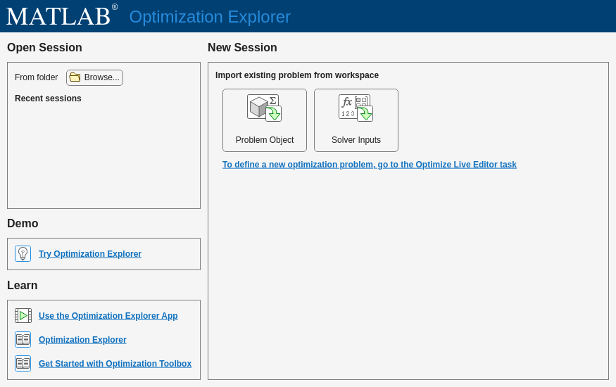
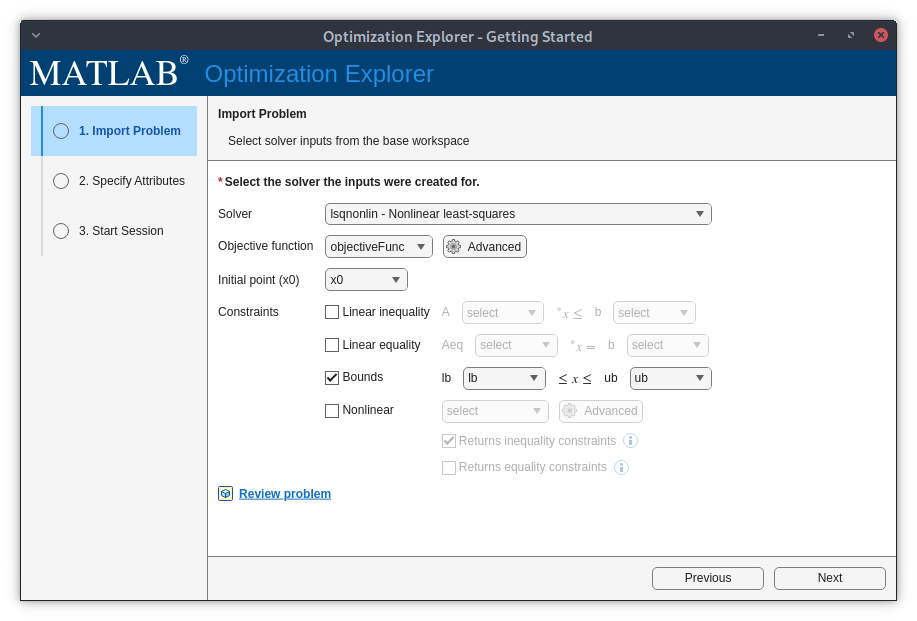
On the app menu, select Solver Inputs in the New Session section. Next, in the Import Problem step, select these options from the dropdown menus. Click Next.

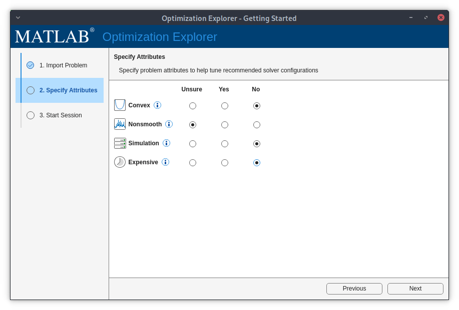
In the Specify Attributes step, check Unsure for the Nonsmooth attribute, as optical optimization problems are typically, but not strictly, nonsmooth. For this optimization problem, check No for the remaining attributes to indicate that the problem is not convex, a simulation, or expensive to compute. Click Next.

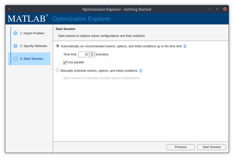
In the Start Session step, check the option to automatically run recommended solvers, and select a small time limit of 10 minutes for the first session only to ensure a correct setup. Check Use parallel if you have access to a parallel computing pool and a Parallel Computing Toolbox™ license. To set up parallel computing for optimization, see Using Parallel Computing in Optimization Toolbox (Optimization Toolbox). Later, you can increase the time limit to probe better designs. To start the optimization session, click Start Session.

While the app is running, click the Show leaderboard button in the Results Table panel to sort the results table in ascending order of the objective value, which is the merit function value. This ensures that the best solution, which will have the lowest objective value, appears in the first row of the table. If you want to pursue further improvements, choose the Manual option to schedule explicit solvers. It is beneficial to run some of the local optimizer solvers using solutions of the global solvers as the starting point. Additionally, using solutions of lsqnonlin as starting points of patternsearch can yield better solutions.

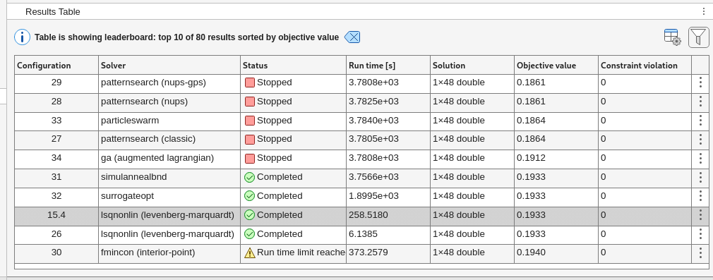
Finally, when the optimization time window is complete, or you have decided the process has converged based on the objective value of each solution displayed in the Results Table, export the sorted table by selecting Export, and then Export Results Table. Save the data table as a variable named explorerResultsTable, which is the default variable name.

Complete optimization results from a session run for 80 minutes using both Auto and Manual modes in a parallel computing environment are stored in the explorerResultsTable variable in a coatingOptimExport.mat file that is attached to this example as a supporting file. Load the results of this optimization session.

load coatingOptimExport

Inspect and Visualize Best Design

After optimization, review the best design candidate. Use the x2opticalCoating helper function to convert the solution vector into an optical coating object. You may also want to examine other top solutions with similar objective values, as they might offer benefits such as reduced sensitivity and improved manufacturing yield.

ind = 1;
oc = x2opticalCoating(explorerResultsTable.Solution{ind},design);

Since manufacturing can only achieve finite precision, round the layer thicknesses to the nearest nanometer to reflect realistic fabrication constraints. To learn more about tolerance and yield analysis, see the Perform Sensitivity and Yield Analysis of Optical Coating Using Monte Carlo example.

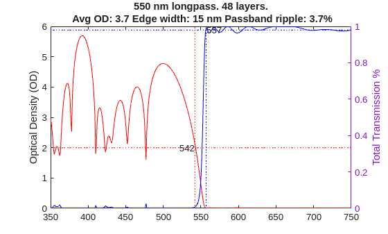
Create a custom plot to assess the optical density, OD, and transmission, Ta, performance of the best filter design.

showLongpassResponse(oc,goals.ODCutOff,goals.TaCutIn);

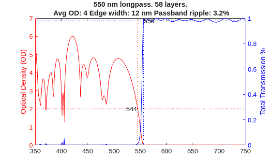
Compare Performance Versus Number of Layers

To evaluate the tradeoff between filter performance and manufacturing cost, compare designs with different numbers of layers (e.g., 18, 28, 38, and 48), using the same materials, thickness constraints, and spectral requirements.

Load the results for each layer count. Observe how increasing the number of layers improves average OD, sharpens the filter edge, and reduces passband ripple. Note that at least 48 layers are needed to achieve less than 5% ripple in the passband, which is a common requirement.

Repeat the visualization for each design to compare their optical performance and assess the impact of layer count on filter characteristics.

load longpass550WithDifferentLayers
figure
showLongpassResponse(oc18l,goals.ODCutOff,goals.TaCutIn)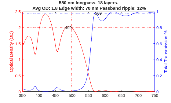

figure
showLongpassResponse(oc28l,goals.ODCutOff,goals.TaCutIn)

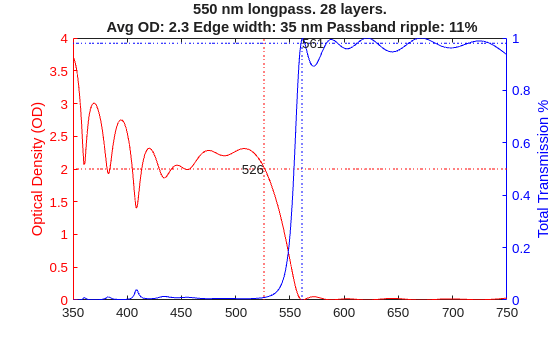
figure
showLongpassResponse(oc38l,goals.ODCutOff,goals.TaCutIn)

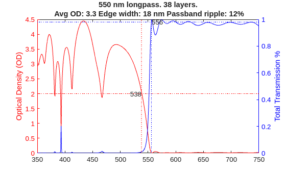
figure
showLongpassResponse(oc,goals.ODCutOff,goals.TaCutIn)

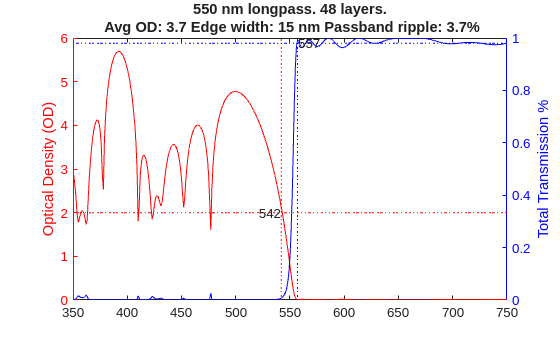
figure
showLongpassResponse(oc58l,goals.ODCutOff,goals.TaCutIn)

Helper Functions

coatingMeritFunc

Compute the total weighted residuals for a candidate optical coating design by quantifying deviations from specified performance goals across multiple spectral bands.

function totres = coatingMeritFunc(oc,goals)
% Return residuals
totres = [];
for bInd = 1:numel(goals.Bands)
    band = goals.Bands(bInd);

    fq = fresnelCoefficients(oc,...
        Wavelengths=band.Wavelengths,...
        IncidentAngles=band.IncidentAngles);
    actResponse = band.ResponseFcn(fq);

    % Check for responses outside the desired lower bound (under-performance)
    lowerres = band.DesiredRange(1) - actResponse;
    % Set residual to zero if performance exceeds lower bound
    lowerres(lowerres < 0) = 0;

    % Check for responses outside the desired upper bound (over-performance/ripple)
    upperres = actResponse - band.DesiredRange(2);
    % Set residual to zero if performance is below upper bound
    upperres(upperres < 0) = 0;

    % Total residual is the sum of any violations
    res = lowerres + upperres;

    % Normalize for number of observations in this band
    res = res.*goals.MaxObservations/numel(res);

    % Apply weights
    res = res.*band.Weight;

    totres = [totres;res(:)]; %#ok<AGROW>   
end
end

x2opticalCoating

Convert a numeric optimization variable to an optical coating object.

function oc = x2opticalCoating(x, design)
oc = opticalCoating(...
    Name=design.Name,...
    PrimaryWavelength=design.PrimaryWavelength,...
    WavelengthRange=design.WavelengthRange,...
    CoatingMaterials=design.Materials,...
    LayerMaterialIndex=design.LayerMaterialIndex,...
    LayerThickness=x,...
    ThicknessUnit="nm",...
    IncidentAngleRange=design.AngleRange,...
    Substrate=design.Substrate);
end

showLongpassResponse

Display the optical density and total transmission response of a longpass filter, highlighting the stopband and passband characteristics, cutoff wavelengths, and relevant performance metrics based on the specified cutoff values.

function showLongpassResponse(oc,ODCutoff,TaCutoff)
fq = fresnelCoefficients(oc,IncidentAngles=0);

lambdas = oc.WavelengthRange(1):oc.WavelengthRange(2);

colororder(["r", "b"])

% Stop band info in red
yyaxis left
od = -log10(fq.Ta);
% The OD plot in red
plot(lambdas,od,'r-');
hold on
% A dotted red line at ODCutOff
plot(lambdas,repmat(ODCutoff,size(lambdas)),'r:');
ylabel("Optical Density (OD)");

% Edge info
% Find last point of OD>ODCutOff
odCutInd = find(od>ODCutoff,1,"last");
wlAtCutOff = lambdas(odCutInd);
% Show as a vertical line
plot([wlAtCutOff,wlAtCutOff],ylim,'r:')
% Display corresponding wavelength (Cut-off wavelength)
text(wlAtCutOff,ODCutoff,num2str(wlAtCutOff),"HorizontalAlignment","right");

% Compute average OD in stop band for display in the title
avgOD = mean(od(1:odCutInd));

% Pass band info in blue
yyaxis right
% Ta plot in blue
plot(lambdas,fq.Ta,'b-');
hold on
% A dotted blue line at Ta Cut off
plot(lambdas,repmat(TaCutoff,size(lambdas)),'b:')
ylabel("Total Transmission %");

% Edge info
% Find first point of T>TaCutoff
tCutInd = find(fq.Ta>TaCutoff,1);
wlAtCutIn = lambdas(tCutInd);
% Show as a vertical line
plot([wlAtCutIn wlAtCutIn],ylim,'b:')
% Cut-in wavelength
text(wlAtCutIn,TaCutoff,num2str(wlAtCutIn),"HorizontalAlignment","left");

% Passband ripple
passBandInds = lambdas>wlAtCutIn;
passBandTa = fq.Ta(passBandInds);
passBandRippleP2P = range(passBandTa);
passBandRippleMean = mean(passBandTa);
passBandRipple = passBandRippleP2P/passBandRippleMean*100;

title("550 nm longpass. "...
    +oc.NumLayers+" layers." ...
    +newline...
    +" Avg OD: "+num2str(avgOD,2)...
    +" Edge width: "+(wlAtCutIn-wlAtCutOff)+" nm"...
    +" Passband ripple: "+num2str(passBandRipple,2)+"%")

end