Narendra-Li ベンチマーク システム: 離散時間システムの非線形グレー ボックス モデリング
このデモでは、入力と出力が 1 つずつある、複雑で人工的な非線形離散時間システムのパラメーターの同定について説明します。システムは以下の文献にある Narendra と Li を元にしています。
  K. S. Narendra and S.-M. Li. "Neural networks in control systems". In
  Mathematical Perspectives on Neural Networks (P. Smolensky,
  M. C. Mozer, and D. E. Rumelhard, eds.), Chapter 11, pages 347-394,
  Lawrence Erlbaum Associates, Hillsdale, NJ, USA, 1996.
また、多数の離散時間同定サンプルで検討されています。
Narendra-Li 離散時間ベンチマーク システム
Narendra-Li システムの離散時間方程式は、次のとおりです。
  x1(t+Ts) = (x1(t)/(1+x1(t)^2)+p(1))*sin(x2(t))
  x2(t+Ts) = x2(t)*cos(x2(t)) + x1(t)*exp(-(x1(t)^2+x2(t)^2)/p(2))
             + u(t)^3/(1+u(t)^2+p(3)*cos(x1(t)+x2(t))
y(t) = x1(t)/(1+p(4)*sin(x2(t))+p(5)*sin(x1(t)))
ここで、x1(t) と x2(t) は状態、u(t) は入力信号、y(t) は出力信号、p は要素が 5 つあるパラメーター ベクトルです。
IDNLGREY 離散時間 Narendra-Li モデル
IDNLGREY モデル ファイルの観点からは、連続時間システムと離散時間システムには違いがありません。したがって、Narendra-Li モデル ファイルは状態更新ベクトル dx および出力 y を返さなければなりません。また、t (時間)、x (状態ベクトル)、u (入力)、p (パラメーター)、varargin を入力引数として受け取ります。
  function [dx, y] = narendrali_m(t, x, u, p, varargin)
  %NARENDRALI_M  A discrete-time Narendra-Li benchmark system.
  % Output equation.
  y = x(1)/(1+p(4)*sin(x(2)))+x(2)/(1+p(5)*sin(x(1)));
  % State equations.
  dx = [(x(1)/(1+x(1)^2)+p(1))*sin(x(2));              ... % State 1.
        x(2)*cos(x(2))+x(1)*exp(-(x(1)^2+x(2)^2)/p(2)) ... % State 2.
           + u(1)^3/(1+u(1)^2+p(3)*cos(x(1)+x(2)))     ...
       ];
5 つのパラメーターすべてを 1 つのパラメーター ベクトルにまとめるよう選択したため、i 番目の成分は MATLAB® での通常の方法、つまり p(i) によって参照できます。
このモデル ファイルを基礎として、次にモデル化の状況を反映させた IDNLGREY オブジェクトを作成します。ここでは、モデルの離散性は Ts の正数で指定されることに注目してください (= 1 秒)。また、パラメーターは 5 行 1 列のパラメーター ベクトルである要素を 1 つだけ維持し、SETPAR を使用してこのベクトルのすべてのコンポーネントが正であることを指定することに注意してください。
FileName      = 'narendrali_m';                    % File describing the model structure.
Order         = [1 1 2];                           % Model orders [ny nu nx].
Parameters    = {[1.05; 7.00; 0.52; 0.52; 0.48]};  % True initial parameters (a vector).
InitialStates = zeros(2, 1);                       % Initial value of initial states.
Ts            = 1;                                 % Time-discrete system with Ts = 1s.
nlgr = idnlgrey(FileName, Order, Parameters, InitialStates, Ts, 'Name', ...
                'Discrete-time Narendra-Li benchmark system',  ...
                'TimeUnit', 's');
nlgr = setpar(nlgr, 'Minimum', {eps(0)*ones(5, 1)});
入力した Narendra-Li モデル構造の概要は、PRESENT コマンドから得られます。
present(nlgr);
nlgr =

Discrete-time nonlinear grey-box model defined by 'narendrali_m' (MATLAB file):

   x(t+Ts) = F(t, x(t), u(t), p1)
      y(t) = H(t, x(t), u(t), p1) + e(t)

 with 1 input(s), 2 state(s), 1 output(s), and 5 free parameter(s) (out of 5).

 Inputs:
    u(1)  (t)
 States:        Initial value
    x(1)  x1(t)   xinit@exp1   0   (fixed) in [-Inf, Inf]
    x(2)  x2(t)   xinit@exp1   0   (fixed) in [-Inf, Inf]
 Outputs:
    y(1)  (t)
 Parameters:    Value
   p1(1)   p1     1.05      (estimated) in ]0, Inf]
   p1(2)             7      (estimated) in ]0, Inf]
   p1(3)          0.52      (estimated) in ]0, Inf]
   p1(4)          0.52      (estimated) in ]0, Inf]
   p1(5)          0.48      (estimated) in ]0, Inf]

Name: Discrete-time Narendra-Li benchmark system
Sample time: 1 seconds

Status:
Created by direct construction or transformation. Not estimated.
More information in model's "Report" property.
入出力データ
それぞれ 300 個のサンプルをもつ 2 つの入出力データ レコードがあり、1 つは推定用、もう 1 つは検証用に使用できます。これらの両方のレコードに使用される入力ベクトルは同一で、2 つの正弦波の和として選択されています。
u(t) = sin(2*pi*t/10) + sin(2*pi*t/25)
ここで、t = 0、1、...、299 秒です。2 つのデータ レコードを保持する 2 つの IDDATA オブジェクトを作成します。ze は推定用、zv は検証用です。
load narendralidata
ze = iddata(y1, u, Ts, 'Tstart', 0, 'Name', 'Narendra-Li estimation data', ...
            'ExperimentName', 'ze');
zv = iddata(y2, u, Ts, 'Tstart', 0, 'Name', 'Narendra-Li validation data', ...
            'ExperimentName', 'zv');
推定に使用される入出力データがプロット ウィンドウに表示されます。
figure('Name', ze.Name);
plot(ze);

図 1: Narendra-Li ベンチマーク システムからの入出力データ
初期 Narendra-Li モデルの性能
今度は、COMPARE を使用して初期 Narendra-Li モデルの性能を調べます。ze および zv のシミュレートされた出力と測定された出力が生成され、既定では ze への適合が表示されます。プロットのコンテキスト メニューを使用して、データの実験を zv に切り替えます。どちらのデータセットも適合は約 74% で悪くありません。ここで、COMPARE は既定の設定で初期状態ベクトルを推定することに注意してください。この場合、ze の 1 つの初期状態ベクトルと zv のベクトルです。
compare(merge(ze, zv), nlgr);

図 2: 初期の Narendra-Li モデルの実際の出力とシミュレーションの出力の比較
%%4
% By looking at the prediction errors obtained via PE, we realize that the
% initial Narendra-Li model shows some systematic and periodic differences
% as compared to the true outputs.
pe(merge(ze, zv), nlgr);
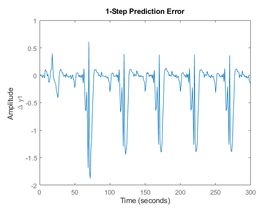
図 3: 初期 Narendra-Li モデルで取得された予測誤差コンテキスト メニューを使用して実験を切り替えます。
パラメーター推定
体系的な不一致を削減するため、Narendra-Li モデル構造の 5 つのすべてのパラメーターを NLGREYEST を使用して推定します。推定は、推定データセット ze のみを使用して実行されます。
opt = nlgreyestOptions('Display', 'on');
nlgr = nlgreyest(ze, nlgr, opt);

推定された Narendra-Li モデルの性能
COMPARE をもう一度使用して推定されたモデルの性能を調べます。今度は、初期状態ベクトル推定をせずに、モデルの内部に保存された初期状態ベクトル (両方の実験で [0; 0]) を使用します。
clf
opt = compareOptions('InitialCondition','m');
compare(merge(ze, zv), nlgr, opt);

図 4: 推定された Narendra-Li モデルの実際の出力とシミュレーションの出力の比較
推定後は大幅な改善が実現し、予測誤差のプロットを参照することでよくわかります。
figure;
pe(merge(ze, zv), nlgr);
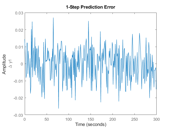
図 5: 推定された Narendra-Li モデルで取得された予測誤差
推定された Narendra-Li モデルのモデル化能力も、RESID による相関解析によって確認されます。
figure('Name', [nlgr.Name ': residuals of estimated model']);
resid(zv, nlgr);

図 6: 推定された Narendra-Li モデルで取得された残差
実際、取得されたモデル パラメーターも実際のモデル出力の生成に使用されたパラメーターと非常に似通っています。
disp('   True      Estimated parameter vector');
ptrue = [1; 8; 0.5; 0.5; 0.5];
fprintf('   %1.4f    %1.4f\n', [ptrue'; getpvec(nlgr)']);
   True      Estimated parameter vector
   1.0000    1.0000
   8.0000    8.0082
   0.5000    0.5003
   0.5000    0.4988
   0.5000    0.5018
次に、いくつかの追加のモデル品質結果 (損失関数、赤池の FPE、モデル パラメーターの推定標準偏差) が、PRESENT コマンドによって提供されます。
present(nlgr);
nlgr =

Discrete-time nonlinear grey-box model defined by 'narendrali_m' (MATLAB file):

   x(t+Ts) = F(t, x(t), u(t), p1)
      y(t) = H(t, x(t), u(t), p1) + e(t)

 with 1 input(s), 2 state(s), 1 output(s), and 5 free parameter(s) (out of 5).

 Inputs:
    u(1)  u1(t)
 States:        Initial value
    x(1)  x1(t)   xinit@exp1   0   (fixed) in [-Inf, Inf]
    x(2)  x2(t)   xinit@exp1   0   (fixed) in [-Inf, Inf]
 Outputs:
    y(1)  y1(t)
 Parameters:       Value Standard Deviation
   p1(1)   p1     0.999993      0.0117615   (estimated) in ]0, Inf]
   p1(2)           8.00821       0.885988   (estimated) in ]0, Inf]
   p1(3)          0.500319      0.0313092   (estimated) in ]0, Inf]
   p1(4)          0.498842       0.264806   (estimated) in ]0, Inf]
   p1(5)          0.501761        0.30998   (estimated) in ]0, Inf]

Name: Discrete-time Narendra-Li benchmark system
Sample time: 1 seconds

Status:
Termination condition: Change in parameters was less than the specified tolerance..
Number of iterations: 16, Number of function evaluations: 17

Estimated using Solver: FixedStepDiscrete; Search: lsqnonlin on time domain data "Narendra-Li estimation data".
Fit to estimation data: 99.44%
FPE: 9.23e-05, MSE: 8.927e-05
More information in model's "Report" property.
連続時間入出力システムの場合、STEP を離散時間入出力システムに使用することもできます。これを 2 つの異なるステップ レベル、1 と 2 に対して実行してみます。
figure('Name', [nlgr.Name ': step responses of estimated model']);
t = (-5:50)';
step(nlgr, 'b', t, stepDataOptions('StepAmplitude',1));
line(t, step(nlgr, t, stepDataOptions('StepAmplitude',2)), 'color', 'g');
grid on;
legend('0 -> 1', '0 -> 2', 'Location', 'NorthWest');
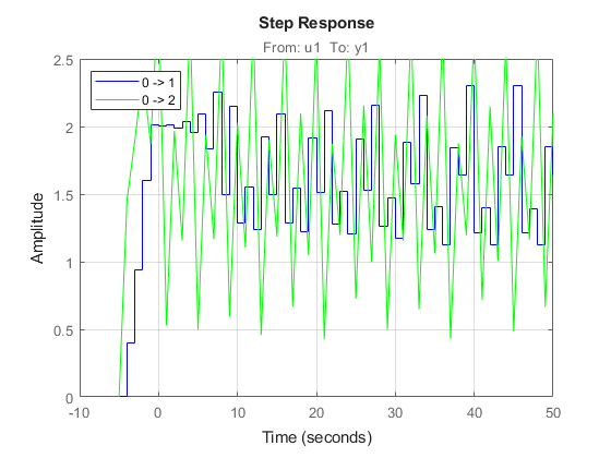
図 7: 推定された Narendra-Li モデルで取得されたステップ応答
最後に、推定された IDNLGREY Narendra-Li モデルの性能をいくつかの基本線形モデルと比較して、この例を終了します。後者のモデルによる一致は、推定された IDNLGREY モデルに返されたものよりも明らかに低くなっています。
nk = delayest(ze);
arx22 = arx(ze, [2 2 nk]);   % Second order linear ARX model.
arx33 = arx(ze, [3 3 nk]);   % Third order linear ARX model.
arx44 = arx(ze, [4 4 nk]);   % Fourth order linear ARX model.
oe22  = oe(ze, [2 2 nk]);    % Second order linear OE model.
oe33  = oe(ze, [3 3 nk]);    % Third order linear OE model.
oe44  = oe(ze, [4 4 nk]);    % Fourth order linear OE model.
clf
fig = gcf;
Pos = fig.Position; fig.Position = [Pos(1:2)*0.7, Pos(3)*1.3, Pos(4)*1.3];
compare(zv, nlgr, 'b', arx22, 'm-', arx33, 'm:', arx44, 'm--', ...
        oe22, 'g-', oe33, 'g:', oe44, 'g--');
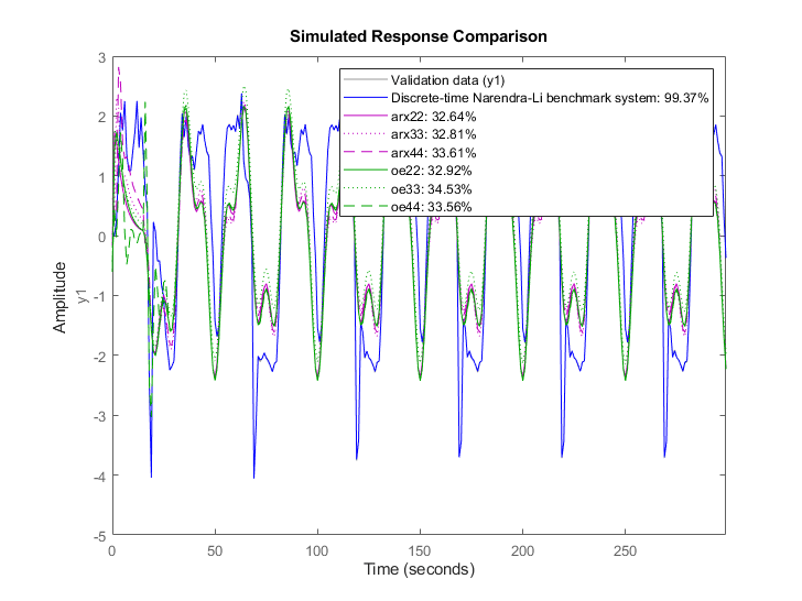
図 8: 複数の Narendra-Li 推定モデルの実際の出力とシミュレーションの出力の比較
まとめ
この例では、架空の Narendra-Li 離散時間ベンチマーク システムを使用して、離散時間 IDNLGREY モデリングの実行の基礎を説明しました。