産業用ロボット アームのモデル化
この例は、産業用ロボット アームのダイナミクスのグレーボックス モデリングを示しています。このロボット アームは、図 1 に示す柔軟な非線形 3 質量モデルで表されます。このモデルは、動きが重力の影響を受けずに軸を中心とすると仮定して理想化されています。簡単にするため、モデル化はギア比 r = 1 でも実行され、実物理パラメーターは後で実ギア比の直接的なスケーリングで取得されます。以下で説明するモデル化と同定実験は、次の文献に基づいています。
  E. Wernholt and S. Gunnarsson. Nonlinear Identification of a
  Physically Parameterized Robot Model. In preprints of the 14th IFAC
  Symposium on System Identification, pages 143-148, Newcastle,
  Australia, March 2006.

図 1: 産業用ロボット アームの概略図
ロボット アームのモデル化
ロボットへの入力は電気モーターから生成される、適用されたトルク u(t)=tau(t) で、結果のモーター角速度 y(t) = d/dt q_m(t) は測定された出力です。ギアボックスの後、およびアーム構造の端にある質量の角度位置 q_g(t) と q_a(t) は、測定不可能です。ギアボックスの柔軟性は非線形バネでモデル化され、バネ トルク tau_s(t) で記述されます。これはモーターと 2 番目の質量の間にあり、最後の 2 つの質量の間にある「線形」バネはアーム構造の柔軟性をモデル化します。システムの摩擦は主に最初の質量に作用し、ここでは非線形摩擦トルク tau_f(t) でモデル化されます。
次の状態を導入します。
         ( x1(t) )   ( q_m(t) - q_g(t) )
         ( x2(t) )   ( q_g(t) - q_a(t) )
  x(t) = ( x3(t) ) = (   d/dt q_m(t)   )
         ( x4(t) )   (   d/dt q_g(t)   )
         ( x5(t) )   (   d/dt q_a(t)   )
トルク バランスを 3 つの質量に適用すると、次の非線形状態空間モデル構造が得られます。
  d/dt x1(t) = x3(t) - x4(t)
  d/dt x2(t) = x4(t) - x5(t)
  d/dt x3(t) = 1/J_m*(-tau_s(t) - d_g*(x3(t)-x4(t)) - tau_f(t) + u(t))
  d/dt x4(t) = 1/J_g*(tau_s(t) + d_g*(x3(t)-x4(t)) - k_a*x2(t) - d_a*(x4(t)-x5(t)))
  d/dt x5(t) = 1/J_a*(k_a*x2(t) + d_a*(x4(t)-x5(t)))
y(t) = x3(t)
ここで、J_m、J_g、J_a はそれぞれモーター、ギアボックス、アーム構造の慣性モーメントで、d_g と d_a は減衰パラメーター、k_a はアーム構造の剛性です。
ギアボックス摩擦トルク tau_f(t) は、実際の摩擦現象の大部分を取り込むようにモデル化されています。特に、クーロン摩擦とストライベック効果を対象としています。
tau_f(t) = Fv*x3(t) + (Fc+Fcs*sech(alpha*x3(t)))*tanh(beta*x3(t))
ここで Fv と Fc は粘性およびクーロン摩擦係数、Fcs と alpha はストライベック効果を反映する係数、beta は速度 x3(t) の負から正への滑らかな移行のために使用されるパラメーターです (速度と摩擦トルク/力の静的関係を記述する、多少モデル構造が異なるが同様のアプローチを、以下のチュートリアル idnlgreydemo5 で説明しています「静的摩擦モデリング」)。
バネのトルク tau_s(t) は、x1(t) に 2 次項のない 3 次多項式で記述されると仮定します。
tau_s(t) = k_g1*x1(t) + k_g3*x1(t)^3
ここで k_g1 と k_g3 は、ギアボックス バネの 2 つの剛性パラメーターです。
Wernholt と Gunnarsson による論文で議論されているその他のタイプの同定実験では、全体的な慣性モーメント J = J_m+J_g+J_a の同定が可能です。これにより、不明なスケーリング係数 a_m と a_g を導入して、次の再パラメーター化を実行できます。
  J_m = J*a_m
  J_g = J*a_g
  J_a = J*(1-a_m-a_g)
ここで (J が既知の場合)、a_m と a_g need のみを推定する必要があります。
総じて、これにより次の状態空間構造が得られ、ここには 13 個の異なるパラメーター が含まれます。Fv、Fc、Fcs、alpha、beta、J、a_m、a_g、k_g1、k_g3、d_g、k_a および d_a 1 (定義により、sech(x) = 1/cosh(x) という事実も使用しています)。
    tau_f(t) = Fv*x3(t) + (Fc+Fcs/cosh(alpha*x3(t)))*tanh(beta*x3(t))
    tau_s(t) = k_g1*x1(t) + k_g3*x1(t)^3
d/dt x1(t) = x3(t) - x4(t) d/dt x2(t) = x4(t) - x5(t) d/dt x3(t) = 1/(J*a_m)*(-tau_s(t) - d_g*(x3(t)-x4(t)) - tau_f(t) + u(t)) d/dt x4(t) = 1/(J*a_g)*(tau_s(t) + d_g*(x3(t)-x4(t)) - k_a*x2(t) - d_a*(x4(t)-x5(t))) d/dt x5(t) = 1/(J(1-a_m-a_g))*(k_a*x2(t) + d_a*(x4(t)-x5(t)))
y(t) = x3(t)
IDNLGREY ロボット アーム モデル オブジェクト
上記のモデル構造は robotarm_c.c という C MEX ファイルに入力され、状態および出力更新関数は次のようになります (ファイル全体はコマンド "type robotarm_c.c" で表示できます)。状態更新関数では、2 つの double 型中間変数を使用しています。1 つは方程式を理解しやすくするため、もう 1 つは実行速度を改善させるためです (taus は方程式に 2 回使用されていますが、1 回だけ計算されます)。
  /* State equations. */
  void compute_dx(double *dx, double *x, double *u, double **p)
  {
      /* Declaration of model parameters and intermediate variables. */
      double *Fv, *Fc, *Fcs, *alpha, *beta, *J, *am, *ag, *kg1, *kg3, *dg, *ka, *da;
      double tauf, taus;   /* Intermediate variables. */
/* Retrieve model parameters. */
Fv = p[0]; /* Viscous friction coefficient. */
Fc = p[1]; /* Coulomb friction coefficient. */
Fcs = p[2]; /* Striebeck friction coefficient. */
alpha = p[3]; /* Striebeck smoothness coefficient. */
beta = p[4]; /* Friction smoothness coefficient. */
J = p[5]; /* Total moment of inertia. */
am = p[6]; /* Motor moment of inertia scale factor. */
ag = p[7]; /* Gear-box moment of inertia scale factor. */
kg1 = p[8]; /* Gear-box stiffness parameter 1. */
kg3 = p[9]; /* Gear-box stiffness parameter 3. */
dg = p[10]; /* Gear-box damping parameter. */
ka = p[11]; /* Arm structure stiffness parameter. */
da = p[12]; /* Arm structure damping parameter. */ /* Determine intermediate variables. */
/* tauf: Gear friction torque. (sech(x) = 1/cosh(x)! */
/* taus: Spring torque. */
tauf = Fv[0]*x[2]+(Fc[0]+Fcs[0]/(cosh(alpha[0]*x[2])))*tanh(beta[0]*x[2]);
taus = kg1[0]*x[0]+kg3[0]*pow(x[0],3); /* x[0]: Rotational velocity difference between the motor and the gear-box. */
/* x[1]: Rotational velocity difference between the gear-box and the arm. */
/* x[2]: Rotational velocity of the motor. */
/* x[3]: Rotational velocity after the gear-box. */
/* x[4]: Rotational velocity of the robot arm. */
dx[0] = x[2]-x[3];
dx[1] = x[3]-x[4];
dx[2] = 1/(J[0]*am[0])*(-taus-dg[0]*(x[2]-x[3])-tauf+u[0]);
dx[3] = 1/(J[0]*ag[0])*(taus+dg[0]*(x[2]-x[3])-ka[0]*x[1]-da[0]*(x[3]-x[4]));
dx[4] = 1/(J[0]*(1.0-am[0]-ag[0]))*(ka[0]*x[1]+da[0]*(x[3]-x[4]));
} /* Output equation. */
void compute_y(double y[], double x[])
{
/* y[0]: Rotational velocity of the motor. */
y[0] = x[2];
}次のステップは、モデル化状況を反映する IDNLGREY オブジェクトを作成することです。ロボット アームの適切な初期パラメーター値を見つけるには、さらに作業が必要なことに注意してください。Wernholt と Gunnarsson の論文では、これは 2 つの先行手順で実行され、その他のモデル構造と同定テクニックが採用されています。以下で使用される初期パラメーター値は、これらの同定実験の結果です。
FileName      = 'robotarm_c';               % File describing the model structure.
Order         = [1 1 5];                    % Model orders [ny nu nx].
Parameters    = [ 0.00986346744839  0.74302635727901 ...
                  3.98628540790595  3.24015074090438 ...
                  0.79943497008153  0.03291699877416 ...
                  0.17910964111956  0.61206166914114 ...
                 20.59269827430799  0.00000000000000 ...
                  0.06241814047290 20.23072060978318 ...
                  0.00987527995798]';       % Initial parameter vector.
InitialStates = zeros(5, 1);                % Initial states.
Ts            = 0;                          % Time-continuous system.
nlgr = idnlgrey(FileName, Order, Parameters, InitialStates, Ts, ...
                'Name', 'Robot arm',                            ...
                'InputName', 'Applied motor torque',            ...
                'InputUnit', 'Nm',                              ...
                'OutputName', 'Angular velocity of motor',      ...
                'OutputUnit', 'rad/s',                          ...
                'TimeUnit', 's');
記録のため、状態の名前と単位を指定します。
nlgr = setinit(nlgr, 'Name', {'Angular position difference between the motor and the gear-box' ...
                       'Angular position difference between the gear-box and the arm'   ...
                       'Angular velocity of motor'                                      ...
                       'Angular velocity of gear-box'                                   ...
                       'Angular velocity of robot arm'}');
nlgr = setinit(nlgr, 'Unit', {'rad' 'rad' 'rad/s' 'rad/s' 'rad/s'});
パラメーター名も詳細に指定します。さらに、モデル化はすべてのパラメーターが正になるように実行されています。つまり、各パラメーターの最小値は 0 に設定されます (このため、制約された推定が後で実行されます)。Wernholt と Gunnarsson の論文にあるように、最初の 6 つのパラメーター (Fv、Fc、Fcs、alpha、beta、J) は良好で推定の必要がないものとします。
nlgr = setpar(nlgr, 'Name', {'Fv   : Viscous friction coefficient'            ... % 1.
                      'Fc   : Coulomb friction coefficient'            ... % 2.
                      'Fcs  : Striebeck friction coefficient'          ... % 3.
                      'alpha: Striebeck smoothness coefficient'        ... % 4.
                      'beta : Friction smoothness coefficient'         ... % 5.
                      'J    : Total moment of inertia'                 ... % 6.
                      'a_m  : Motor moment of inertia scale factor'    ... % 7.
                      'a_g  : Gear-box moment of inertia scale factor' ... % 8.
                      'k_g1 : Gear-box stiffness parameter 1'          ... % 9.
                      'k_g3 : Gear-box stiffness parameter 3'          ... % 10.
                      'd_g  : Gear-box damping parameter'              ... % 11.
                      'k_a  : Arm structure stiffness parameter'       ... % 12.
                      'd_a  : Arm structure damping parameter'         ... % 13.
                     });
nlgr = setpar(nlgr, 'Minimum', num2cell(zeros(size(nlgr, 'np'), 1)));   % All parameters >= 0!
for parno = 1:6   % Fix the first six parameters.
    nlgr.Parameters(parno).Fixed = true;
end
ここまで実行したモデル化ステップにより、次のプロパティの初期ロボット アーム モデルが得られました。
present(nlgr);
nlgr =

Continuous-time nonlinear grey-box model defined by 'robotarm_c' (MEX-file):

   dx/dt = F(t, x(t), u(t), p1, ..., p13)
    y(t) = H(t, x(t), u(t), p1, ..., p13) + e(t)

 with 1 input(s), 5 state(s), 1 output(s), and 7 free parameter(s) (out of 13).

 Inputs:
    u(1)   Applied motor torque(t) [Nm]
 States:                                                                           Initial value
    x(1)   Angular position difference between the motor and the gear-box(t) [rad]   xinit@exp1   0   (fixed) in [-Inf, Inf]
    x(2)   Angular position difference between the gear-box and the arm(t) [rad]     xinit@exp1   0   (fixed) in [-Inf, Inf]
    x(3)   Angular velocity of motor(t) [rad/s]                                      xinit@exp1   0   (fixed) in [-Inf, Inf]
    x(4)   Angular velocity of gear-box(t) [rad/s]                                   xinit@exp1   0   (fixed) in [-Inf, Inf]
    x(5)   Angular velocity of robot arm(t) [rad/s]                                  xinit@exp1   0   (fixed) in [-Inf, Inf]
 Outputs:
    y(1)   Angular velocity of motor(t) [rad/s]
 Parameters:                                             Value
    p1    Fv   : Viscous friction coefficient                0.00986347      (fixed) in [0, Inf]
    p2    Fc   : Coulomb friction coefficient                  0.743026      (fixed) in [0, Inf]
    p3    Fcs  : Striebeck friction coefficient                 3.98629      (fixed) in [0, Inf]
    p4    alpha: Striebeck smoothness coefficient               3.24015      (fixed) in [0, Inf]
    p5    beta : Friction smoothness coefficient               0.799435      (fixed) in [0, Inf]
    p6    J    : Total moment of inertia                       0.032917      (fixed) in [0, Inf]
    p7    a_m  : Motor moment of inertia scale factor           0.17911      (estimated) in [0, Inf]
    p8    a_g  : Gear-box moment of inertia scale factor       0.612062      (estimated) in [0, Inf]
    p9    k_g1 : Gear-box stiffness parameter 1                 20.5927      (estimated) in [0, Inf]
    p10   k_g3 : Gear-box stiffness parameter 3                       0      (estimated) in [0, Inf]
    p11   d_g  : Gear-box damping parameter                   0.0624181      (estimated) in [0, Inf]
    p12   k_a  : Arm structure stiffness parameter              20.2307      (estimated) in [0, Inf]
    p13   d_a  : Arm structure damping parameter             0.00987528      (estimated) in [0, Inf]

Name: Robot arm

Status:
Created by direct construction or transformation. Not estimated.
More information in model's "Report" property.
入出力データ
実世界のデータセットの大部分は、実験ロボットから収集されています。ロボットを動作点付近に維持し、安全性の理由から、データは実験的フィードバック制御手段を使用して収集され、これによってジョイント コントローラーの基準信号をオフラインで計算できます。
このケース スタディでは、今後の議論を 4 つの異なるデータセットに絞ります。1 つは推定用、残りは検証用です。それぞれの場合、約 10 秒間の定期的な励起信号が導入され、コントローラーの基準速度を生成します。選択されたサンプリング周波数は 2 kHz です (サンプル時間 Ts = 0.0005 秒)。データセットでは、3 つの異なる種類の入力信号が使用されました (ue: 推定データセットの入力信号。uv1、uv2、uv3: 3 つの検証データセットの入力信号)
  ue, uv1: Multisine signals with a flat amplitude spectrum in the
           frequency interval 1-40 Hz with a peak value of 16 rad/s. The
           multisine signal is superimposed on a filtered square wave
           with amplitude 20 rad/s and cut-off frequency 1 Hz.
uv2: Similar to ue and uv1, but without the square wave.
      uv3: Multisine signal (sum of sinusoids) with frequencies 0.1,
           0.3, and 0.5 Hz, with peak value 40 rad/s.
使用できるデータを読み込んで、すべての 4 つのデータセットを 1 つの IDDATA オブジェクト z に取り込みます。
load('robotarmdata');
z = iddata({ye yv1 yv2 yv3}, {ue uv1 uv2 uv3}, 0.5e-3, 'Name', 'Robot arm');
z.InputName = 'Applied motor torque';
z.InputUnit = 'Nm';
z.OutputName = 'Angular velocity of motor';
z.OutputUnit = 'rad/s';
z.ExperimentName = {'Estimation' 'Validation 1'  'Validation 2' 'Validation 3'};
z.Tstart = 0;
z.TimeUnit = 's';
present(z);
th =

Time domain data set containing 4 experiments.

Experiment                      Samples      Sample Time
   Estimation                    19838            0.0005
   Validation 1                  19838            0.0005
   Validation 2                  19838            0.0005
   Validation 3                  19838            0.0005

Name: Robot arm

Outputs                         Unit (if specified)
   Angular velocity of motor       rad/s

Inputs                          Unit (if specified)
   Applied motor torque            Nm
次の図は、4 つの実験で使用される入出力データを示します。
figure('Name', [z.Name ': input-output data'],...
   'DefaultAxesTitleFontSizeMultiplier',1,...
   'DefaultAxesTitleFontWeight','normal',...
   'Position',[100 100 900 600]);
ne = size(z,'ne');
for i = 1:ne
    zi = getexp(z, i);
    subplot(ne, 2, 2*i-1);   % Input.
    plot(zi.u);
    title([z.ExperimentName{i} ': ' zi.InputName{1}],'FontWeight','normal');
    if (i < ne)
        xlabel('');
    else
        xlabel([z.Domain ' (' zi.TimeUnit ')']);
    end
    subplot(ne, 2, 2*i);     % Output.
    plot(zi.y);
    title([z.ExperimentName{i} ': ' zi.OutputName{1}],'FontWeight','normal');
    if (i < ne)
        xlabel('');
    else
        xlabel([z.Domain ' (' zi.TimeUnit ')']);
    end
end
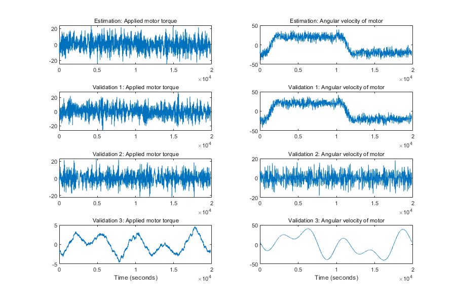
図 2: 実験ロボット アームの測定された入出力データ
初期ロボット アーム モデルの性能
初期ロボット アーム モデルはどの程度良好でしょうか。COMPARE を使用してモデル出力 (4 つの実験すべて) をシミュレートし、結果を対応する測定された出力と比較してみます。4 つのすべての実験について、最初の 2 つの状態の値が 0 (固定) で、残りの 3 つの状態の値が開始時に最初は測定された出力 (固定されていない) に設定されていることがわかっています。ただし、既定の設定では COMPARE はすべての初期状態を推定し、z は 4 つの異なる実験を保持するため、4*5 = 20 個の初期状態を推定することになります。最初の 2 つの状態を固定した後でも、推定対象として 4*3 = 12 個の初期状態が残ります (内部モデル初期状態戦略に従う場合)。データセットは比較的大きいため、計算時間が長くなります。また、これを防止するため、PREDICT を使用して 4*3 個の自由コンポーネントを推定しますが (初期状態が初期状態構造として渡される場合に可能)、推定を最初の 10 個のデータに制限します。次に、COMPARE を使用して、結果の 5 行 4 列の初期状態行列 X0init を初期状態推定を実行せずに使用します。
Ns = size(zi,1);
zred = z(1:round(Ns/10));
nlgr = setinit(nlgr, 'Fixed', {true true false false false});
X0 = nlgr.InitialStates;
[X0.Value] = deal(zeros(1, 4), zeros(1, 4), [ye(1) yv1(1) yv2(1) yv3(1)], ...
    [ye(1) yv1(1) yv2(1) yv3(1)], [ye(1) yv1(1) yv2(1) yv3(1)]);
[~, X0init] = predict(zred, nlgr, [], X0);
nlgr = setinit(nlgr, 'Value', num2cell(X0init(:, 1)));
clf
compare(z, nlgr, [], compareOptions('InitialCondition', X0init));
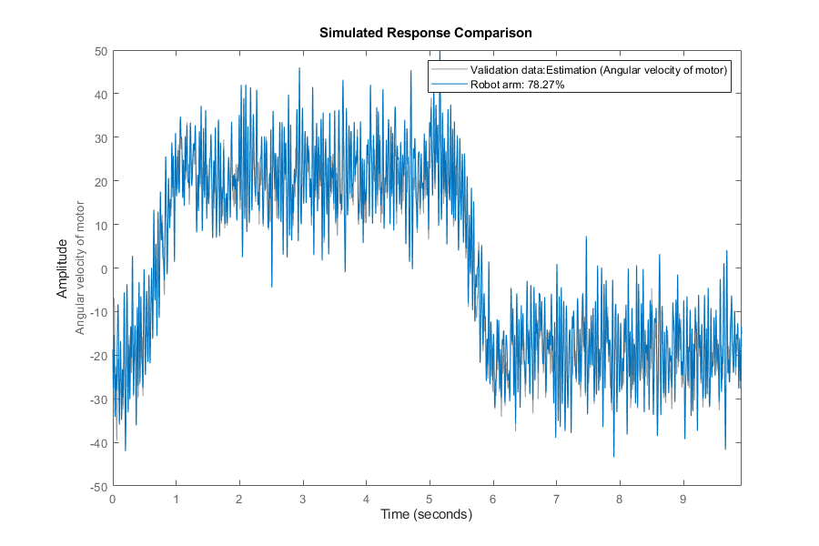
図 3: 初期ロボット アーム モデルの測定された出力とシミュレーションの出力の比較
わかるように、初期ロボット アーム モデルの性能は良好です。3 つの種類のデータセットの適合は、ye と yv1 では約 79%、yv2 では 37%、yv3 では 95% です。ye/yv1 のほうが yv2 よりも適合が高いのは、主に初期モデルの矩形波を取り込む能力によるものです。一方で、多重正弦波部分は等しく取り込まれません。4 つの実験の予測誤差についても検討できます。
pe(z, nlgr, peOptions('InitialCondition',X0init));
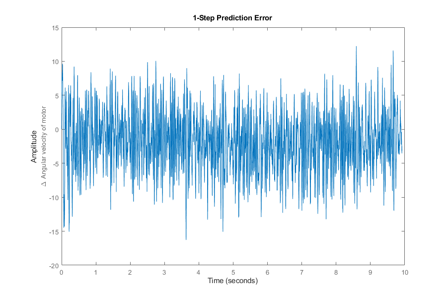
図 4: 初期ロボット アーム モデルの予測誤差
パラメーター推定
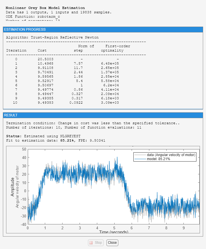
今度は、最初の実験 z (推定データセット) の 7 つの自由モデル パラメーターと 3 つの自由初期状態を推定して、初期ロボット アーム モデルの性能を向上させます。この推定には時間がかかります (通常数分)。
nlgr = nlgreyest(nlgr, getexp(z, 1), nlgreyestOptions('Display', 'on'));
推定されたロボット アーム モデルの性能
COMPARE を再度使用して、推定されたロボット アーム モデルの性能を評価します。ここでは、COMPARE にいかなる初期状態評価も実行しないように指示します。最初の実験では、推測した初期状態を NLGREYEST で推定した状態で置き換え、残りの 3 つの実験では PREDICT を使用して、縮小した IDDATA オブジェクト zred に基づいて初期状態を推定します。
X0init(:, 1) = cell2mat(getinit(nlgr, 'Value'));
X0 = nlgr.InitialStates;
[X0.Value] = deal(zeros(1, 3), zeros(1, 3), [yv1(1) yv2(1) yv3(1)], ...
    [yv1(1) yv2(1) yv3(1)], [yv1(1) yv2(1) yv3(1)]);
[yp, X0init(:, 2:4)] = predict(getexp(zred, 2:4), nlgr, [], X0);
clf
compare(z, nlgr, [], compareOptions('InitialCondition', X0init));
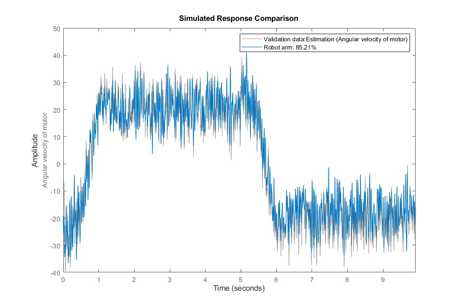
図 5: 推定されたロボット アーム モデルの測定された出力とシミュレーションの出力の比較
比較プロットに、適合の向上という改善が示されます。ye と yv1 の適合は約 85% になり (以前は 79%)、yv2 は約 63% に (以前は 37%)、yv3 は 95.5% よりやや小さく (以前も 95.5% 弱) なっています。改善は 2 番目の検証データセットで最も顕著で、矩形波のない多重正弦波信号が入力として適用されました。ただし、ye と yv1 の多重正弦波部分を取り込む推定されたモデルの能力は、かなり改善されています (矩形波への適合の影響を強く受けるため、これは適合の図には反映されていません)。予測誤差のプロットから、残差は初期ロボット アーム モデルよりも一般に小さくなったことがわかります。
figure;
pe(z, nlgr, peOptions('InitialCondition',X0init));
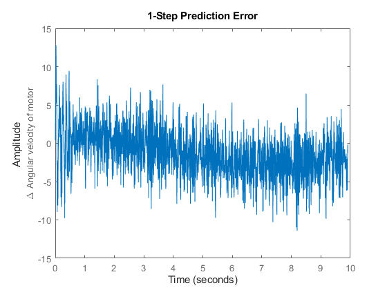
図 6: 推定されたロボット アーム モデルの予測誤差
このケース スタディの最後に、推定されたロボット アーム モデルのさまざまなプロパティをテキスト形式でまとめます。
present(nlgr);
nlgr =

Continuous-time nonlinear grey-box model defined by 'robotarm_c' (MEX-file):

   dx/dt = F(t, x(t), u(t), p1, ..., p13)
    y(t) = H(t, x(t), u(t), p1, ..., p13) + e(t)

 with 1 input(s), 5 state(s), 1 output(s), and 7 free parameter(s) (out of 13).

 Inputs:
    u(1)   Applied motor torque(t) [Nm]
 States:                                                                           Initial value
    x(1)   Angular position difference between the motor and the gear-box(t) [rad]   xinit@exp1          0   (fixed) in [-Inf, Inf]
    x(2)   Angular position difference between the gear-box and the arm(t) [rad]     xinit@exp1          0   (fixed) in [-Inf, Inf]
    x(3)   Angular velocity of motor(t) [rad/s]                                      xinit@exp1   -19.0688   (estimated) in [-Inf, Inf]
    x(4)   Angular velocity of gear-box(t) [rad/s]                                   xinit@exp1   -22.2343   (estimated) in [-Inf, Inf]
    x(5)   Angular velocity of robot arm(t) [rad/s]                                  xinit@exp1   -23.4242   (estimated) in [-Inf, Inf]
 Outputs:
    y(1)   Angular velocity of motor(t) [rad/s]
 Parameters:                                                Value   Standard Deviation
    p1    Fv   : Viscous friction coefficient                0.00986347                0   (fixed) in [0, Inf]
    p2    Fc   : Coulomb friction coefficient                  0.743026                0   (fixed) in [0, Inf]
    p3    Fcs  : Striebeck friction coefficient                 3.98629                0   (fixed) in [0, Inf]
    p4    alpha: Striebeck smoothness coefficient               3.24015                0   (fixed) in [0, Inf]
    p5    beta : Friction smoothness coefficient               0.799435                0   (fixed) in [0, Inf]
    p6    J    : Total moment of inertia                       0.032917                0   (fixed) in [0, Inf]
    p7    a_m  : Motor moment of inertia scale factor          0.266479      0.000286923   (estimated) in [0, Inf]
    p8    a_g  : Gear-box moment of inertia scale factor       0.647533      0.000190954   (estimated) in [0, Inf]
    p9    k_g1 : Gear-box stiffness parameter 1                 20.0774        0.0263501   (estimated) in [0, Inf]
    p10   k_g3 : Gear-box stiffness parameter 3                  24.178         0.332319   (estimated) in [0, Inf]
    p11   d_g  : Gear-box damping parameter                    0.030513      0.000282694   (estimated) in [0, Inf]
    p12   k_a  : Arm structure stiffness parameter              11.7552        0.0311121   (estimated) in [0, Inf]
    p13   d_a  : Arm structure damping parameter             0.00283465      8.05161e-05   (estimated) in [0, Inf]

Name: Robot arm

Status:
Termination condition: Change in cost was less than the specified tolerance..
Number of iterations: 10, Number of function evaluations: 11

Estimated using Solver: ode45; Search: lsqnonlin on time domain data "Robot arm".
Fit to estimation data: 85.21%
FPE: 9.503, MSE: 9.494
More information in model's "Report" property.
結果のまとめ
システム同定テクニックはロボティクスで広く使用されています。「良好」なロボット モデルは、現代のロボット制御コンセプトにとって重要で、速度と精度を常に向上させるために不可欠なものと考えられています。モデルはさまざまなロボット診断アプリケーションで重要なコンポーネントでもあり、モデルは摩耗に関連する問題の予測や、ロボット誤作動の実際の原因の検出に使用されます。