System Identification Toolbox を使用したプロセス モデルの構築と推定
この例では、System Identification Toolbox™ を使用して、シンプルなプロセス モデルを構築する方法を説明します。このようなモデルを作成し、実験データを使用してそのパラメーターを推定する手法を説明します。この例では Simulink® が必要です。
はじめに
この例では、プロセス業界で一般的に使用されるシンプルなプロセス モデルを構築する方法について説明します。プロセス動作を記述するには、通常、シンプルで低次数の連続時間伝達関数を使用します。このようなモデルは、伝達関数を極-零点-ゲインの形式で表す IDPROC オブジェクトを使用して記述できます。
プロセス モデルは、基本タイプ "静的ゲイン + 時定数 + 時間遅延" となります。以下のように、表現できます。

あるいは、積分プロセスとして表現されます:
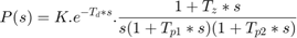
ここで、ユーザーは、実極数 (0、1、2 または 3)、分子での零点の存在、積分器項の存在 (1/s)、および時間遅延の存在 (Td) を設定できます。また、極の不足減衰 (複素数) ペアを実極と置き換えることができます。
IDPROC オブジェクトを使用したプロセス モデルの表現
IDPROC オブジェクトは、文字 P (プロセス モデル)、D (時間遅延)、Z (零点) および I (積分器) を使用してプロセス モデルを定義します。整数は、極数を示します。モデルは、これらの文字で作成された文字ベクトルを含む idproc を呼び出して生成されます。
以下に例を示します。
idproc('P1') % transfer function with only one pole (no zeros or delay)
idproc('P2DIZ') % model with 2 poles, delay integrator and delay
idproc('P0ID') % model with no poles, but an integrator and a delay
ans =

Process model with transfer function:
             Kp
  G(s) = ----------
          1+Tp1*s

        Kp = NaN
       Tp1 = NaN

Parameterization:
    {'P1'}
   Number of free coefficients: 2
   Use "getpvec", "getcov" for parameters and their uncertainties.

Status:
Created by direct construction or transformation. Not estimated.


ans =

Process model with transfer function:
                   1+Tz*s
  G(s) = Kp * ------------------- * exp(-Td*s)
              s(1+Tp1*s)(1+Tp2*s)

         Kp = NaN
        Tp1 = NaN
        Tp2 = NaN
         Td = NaN
         Tz = NaN

Parameterization:
    {'P2DIZ'}
   Number of free coefficients: 5
   Use "getpvec", "getcov" for parameters and their uncertainties.

Status:
Created by direct construction or transformation. Not estimated.


ans =

Process model with transfer function:
          Kp
  G(s) = --- * exp(-Td*s)
          s

        Kp = NaN
        Td = NaN

Parameterization:
    {'P0DI'}
   Number of free coefficients: 2
   Use "getpvec", "getcov" for parameters and their uncertainties.

Status:
Created by direct construction or transformation. Not estimated.
IDPROC オブジェクトの作成 (Simulink モデルを例として使用)
以下の Simulink モデルで記述されるシステムを見てみましょう。
open_system('iddempr1')
set_param('iddempr1/Random Number','seed','0')

赤い部分はシステム、青い部分はコントローラー、基準信号はスイープ正弦波 (チャープ信号) です。データのサンプル時間は 0.5 秒に設定されます。前述のように、システムは連続時間伝達関数であり、idss、idpoly または idproc など、System Identification Toolbox のモデル オブジェクトを使用して記述できます。
idpoly および idproc オブジェクトを使用して、システムを記述してみます。idpoly オブジェクトを使用して、システムは以下のように記述できます。
m0 = idpoly(1,0.1,1,1,[1 0.5],'Ts',0,'InputDelay',1.57,'NoiseVariance',0.01);
上記のような IDPOLY 形式の使用は、任意の次数の伝達関数を記述するときに便利です。ここで検討しているシステムは、非常にシンプルで (1 極、零点なし)、連続時間であるため、よりシンプルな IDPROC オブジェクトを使用してそのダイナミクスを捕捉できます。
m0p = idproc('p1d','Kp',0.2,'Tp1',2,'Td',1.57) % one pole+delay, with initial values
                                               % for gain, pole and delay specified.
m0p =

Process model with transfer function:
             Kp
  G(s) = ---------- * exp(-Td*s)
          1+Tp1*s

        Kp = 0.2
       Tp1 = 2
        Td = 1.57

Parameterization:
    {'P1D'}
   Number of free coefficients: 3
   Use "getpvec", "getcov" for parameters and their uncertainties.

Status:
Created by direct construction or transformation. Not estimated.
IDPROC モデルのパラメーターの推定
システムを、IDPROC などのモデル オブジェクトで記述したら、測定データを使用して、そのパラメーターの推定に使用できます。例として、シミュレーション データを使用して、Simulink モデルのシステム (赤い部分) のパラメーターを推定するときの問題を考えてみます。推定に使用するデータをまず取得します。
sim('iddempr1')
dat1e = iddata(y,u,0.5); % The IDDATA object for storing measurement data
データをよく見てください。
plot(dat1e)

IDPROC モデルを作成するときに指定したのと同じ構造情報に基づいて、procest コマンドを使ってプロセス モデルを特定できます。たとえば、1 極 + 遅延モデルは、以下のように procest を呼び出して推定できます。
m1 = procest(dat1e,'p1d'); % estimation of idproc model using data 'dat1e'.

% Check the result of estimation:
m1
m1 =

Process model with transfer function:
             Kp
  G(s) = ---------- * exp(-Td*s)
          1+Tp1*s

        Kp = 0.20045
       Tp1 = 2.0431
        Td = 1.499

Parameterization:
    {'P1D'}
   Number of free coefficients: 3
   Use "getpvec", "getcov" for parameters and their uncertainties.

Status:
Estimated using PROCEST on time domain data "dat1e".
Fit to estimation data: 87.34%
FPE: 0.01069, MSE: 0.01062
To get information about uncertainties, use
present(m1)
m1 =

Process model with transfer function:
             Kp
  G(s) = ---------- * exp(-Td*s)
          1+Tp1*s

        Kp = 0.20045 +/- 0.00077275
       Tp1 = 2.0431 +/- 0.061216
        Td = 1.499 +/- 0.040854

Parameterization:
    {'P1D'}
   Number of free coefficients: 3
   Use "getpvec", "getcov" for parameters and their uncertainties.

Status:
Termination condition: Near (local) minimum, (norm(g) < tol)..
Number of iterations: 4, Number of function evaluations: 9

Estimated using PROCEST on time domain data "dat1e".
Fit to estimation data: 87.34%
FPE: 0.01069, MSE: 0.01062
More information in model's "Report" property.
モデル パラメーター K、Tp1、および Td と、標準偏差 1 の不確かさの範囲を示します。
IDPROC モデルの時間および周波数応答の算出
前述のように推定した m1 は、すべてのツールボックスのモデル コマンドを適用できる IDPROC モデル オブジェクトです。
step(m1,m0) %step response of models m1 (estimated) and m0 (actual)
legend('m1 (estimated parameters)','m0 (known parameters)','location','northwest')

信頼領域が標準偏差 3 に対応するボード応答は、以下のように算出できます。
h = bodeplot(m1,m0);
showConfidence(h,3)

同様に、以下のように compare を使用して、測定データをモデル出力と比較できます。
compare(dat1e,m0,m1)

sim、impulse、c2d などの処理も、他のモデル オブジェクトと同じように使用できます。
bdclose('iddempr1')
推定でサンプル間動作の作用の適応
入力データのサンプル間動作を評価することが (少なくともスロー サンプリングの場合) 重要となることがあります。これを理解するため、前述と同じシステムを、サンプル アンド ホールド回路なしで確認します。
open_system('iddempr5')

このシステムを同じサンプル時間でシミュレートします。
sim('iddempr5')
dat1f = iddata(y,u,0.5); % The IDDATA object for the simulated data
data1f を使用して IDPROC モデルを推定し、許容される値の遅延の上限も設定します。検索方法として "lm" を使用し、さらに推定の進捗状況を表示します。
m2_init = idproc('P1D');
m2_init.Structure.Td.Maximum = 2;
opt = procestOptions('SearchMethod','lm','Display','on');
m2 = procest(dat1f,m2_init,opt);
m2
m2 =

Process model with transfer function:
             Kp
  G(s) = ---------- * exp(-Td*s)
          1+Tp1*s

        Kp = 0.20038
       Tp1 = 2.01
        Td = 1.31

Parameterization:
    {'P1D'}
   Number of free coefficients: 3
   Use "getpvec", "getcov" for parameters and their uncertainties.

Status:
Estimated using PROCEST on time domain data "dat1f".
Fit to estimation data: 87.26%
FPE: 0.01067, MSE: 0.01061

このモデルは、以前のモデル m1 よりも遅延の推定の精度が若干低くなっています。
[m0p.Td, m1.Td, m2.Td]
step(m0,m1,m2)
legend('m0 (actual)','m1 (estimated with ZOH)','m2 (estimated without ZOH)','location','southeast')
ans =

    1.5700    1.4990    1.3100

ただし、サンプル間動作が 1 次ホールド (実連続の近似値) 入力である推定プロセスを見ると、さらに改善が見込めます。
dat1f.InterSample = 'foh';
m3 = procest(dat1f,m2_init,opt);

4 つのモデル m0 (実)、m1 (zoh 入力から取得)、m2 (連続入力から取得、zoh 想定)、および m3 (同じ入力から取得、ただし foh 想定) を比較します。
[m0p.Td, m1.Td, m2.Td, m3.Td]
compare(dat1e,m0,m1,m2,m3)
ans =

    1.5700    1.4990    1.3100    1.5570

step(m0,m1,m2,m3)
legend('m0','m1','m2','m3')
bdclose('iddempr5')

閉ループで動作するシステムのモデル化
ここでは、閉ループで動作する、統合による複雑なプロセスを検討します。
open_system('iddempr2')

真のシステムは、以下のように表現できます。
m0 = idproc('P2ZDI','Kp',1,'Tp1',1,'Tp2',5,'Tz',3,'Td',2.2);
プロセスは制限された入力振幅と 0 次ホールド デバイス付きの PD 制御器により制御されます。サンプル時間は 1 秒です。
set_param('iddempr2/Random Number','seed','0')
sim('iddempr2')
dat2 = iddata(y,u,1); % IDDATA object for estimation
1 つは推定、もう 1 つは検証のため、異なる 2 つのシミュレーションを行います。
set_param('iddempr2/Random Number','seed','13')
sim('iddempr2')
dat2v = iddata(y,u,1); % IDDATA object for validation purpose
データをご覧ください (推定と検証)。
plot(dat2,dat2v)
legend('dat2 (estimation)','dat2v (validation)')

dat2 を使用して、推定を行います。
Warn = warning('off','Ident:estimation:underdampedIDPROC');
m2_init = idproc('P2ZDI');
m2_init.Structure.Td.Maximum = 5;
m2_init.Structure.Tp1.Maximum = 2;
opt = procestOptions('SearchMethod','lsqnonlin','Display','on');
opt.SearchOptions.MaxIterations  = 100;
m2 = procest(dat2, m2_init, opt)
m2 =

Process model with transfer function:
                   1+Tz*s
  G(s) = Kp * ------------------- * exp(-Td*s)
              s(1+Tp1*s)(1+Tp2*s)

         Kp = 0.98412
        Tp1 = 2
        Tp2 = 1.4838
         Td = 1.713
         Tz = 0.027244

Parameterization:
    {'P2DIZ'}
   Number of free coefficients: 5
   Use "getpvec", "getcov" for parameters and their uncertainties.

Status:
Estimated using PROCEST on time domain data "dat2".
Fit to estimation data: 91.51%
FPE: 0.1128, MSE: 0.1092

compare(dat2v,m2,m0) % Gives very good agreement with data

bode(m2,m0)
legend({'m2 (est)','m0 (actual)'},'location','west')

impulse(m2,m0)
legend({'m2 (est)','m0 (actual)'})

真のシステムのパラメーターとも比較します。
present(m2)
[getpvec(m0), getpvec(m2)]
m2 =

Process model with transfer function:
                   1+Tz*s
  G(s) = Kp * ------------------- * exp(-Td*s)
              s(1+Tp1*s)(1+Tp2*s)

         Kp = 0.98412 +/- 0.013672
        Tp1 = 2 +/- 8.2231
        Tp2 = 1.4838 +/- 10.193
         Td = 1.713 +/- 63.703
         Tz = 0.027244 +/- 65.516

Parameterization:
    {'P2DIZ'}
   Number of free coefficients: 5
   Use "getpvec", "getcov" for parameters and their uncertainties.

Status:
Termination condition: Change in cost was less than the specified tolerance..
Number of iterations: 3, Number of function evaluations: 4

Estimated using PROCEST on time domain data "dat2".
Fit to estimation data: 91.51%
FPE: 0.1128, MSE: 0.1092
More information in model's "Report" property.


ans =

    1.0000    0.9841
    1.0000    2.0000
    5.0000    1.4838
    2.2000    1.7130
    3.0000    0.0272
注意。いくつかのリアルタイム定数の同定は、特にデータを閉ループで収集する場合、悪条件の問題になることがあります。
これを説明するため、検証データに基づいてモデルを推定します。
m2v = procest(dat2v, m2_init, opt)
[getpvec(m0), getpvec(m2), getpvec(m2v)]
m2v =

Process model with transfer function:
                   1+Tz*s
  G(s) = Kp * ------------------- * exp(-Td*s)
              s(1+Tp1*s)(1+Tp2*s)

         Kp = 0.95747
        Tp1 = 1.999
        Tp2 = 0.60819
         Td = 2.314
         Tz = 0.0010561

Parameterization:
    {'P2DIZ'}
   Number of free coefficients: 5
   Use "getpvec", "getcov" for parameters and their uncertainties.

Status:
Estimated using PROCEST on time domain data "dat2v".
Fit to estimation data: 90.65%
FPE: 0.1397, MSE: 0.1353


ans =

    1.0000    0.9841    0.9575
    1.0000    2.0000    1.9990
    5.0000    1.4838    0.6082
    2.2000    1.7130    2.3140
    3.0000    0.0272    0.0011

このモデルは、パラメーター値の状態がよくありません。しかし、他のデータセット dat2 でテストした場合、真のシステム m0 とほぼ同じように動作します。
compare(dat2,m0,m2,m2v)

推定中における既知のパラメーターの固定
他のソースから、1 つの時定数が 1 であることが判明していると想定します。
m2v.Structure.Tp1.Value = 1;
m2v.Structure.Tp1.Free = false;
この値を固定して、以下のように他のパラメーターを推定できます
m2v = procest(dat2v,m2v)
%
m2v =

Process model with transfer function:
                   1+Tz*s
  G(s) = Kp * ------------------- * exp(-Td*s)
              s(1+Tp1*s)(1+Tp2*s)

         Kp = 1.0111
        Tp1 = 1
        Tp2 = 5.3014
         Td = 2.195
         Tz = 3.231

Parameterization:
    {'P2DIZ'}
   Number of free coefficients: 4
   Use "getpvec", "getcov" for parameters and their uncertainties.

Status:
Estimated using PROCEST on time domain data "dat2v".
Fit to estimation data: 92.05%
FPE: 0.09952, MSE: 0.09794

前述のように、Tp1 を既知の値に固定すると、モデル m2v での残りのパラメーターの推定が劇的に改善されます。
また、シンプルな近似がこのデータで有効であることもわかります。
m1x_init = idproc('P2D'); % simpler structure (no zero, no integrator)
m1x_init.Structure.Td.Maximum = 2;
m1x = procest(dat2v, m1x_init)
compare(dat2,m0,m2,m2v,m1x)
m1x =

Process model with transfer function:
                Kp
  G(s) = ----------------- * exp(-Td*s)
         (1+Tp1*s)(1+Tp2*s)

         Kp = -0.8956
        Tp1 = 1.025e-06
        Tp2 = 0.0047599
         Td = 2

Parameterization:
    {'P2D'}
   Number of free coefficients: 4
   Use "getpvec", "getcov" for parameters and their uncertainties.

Status:
Estimated using PROCEST on time domain data "dat2v".
Fit to estimation data: -24.18%
FPE: 24.27, MSE: 23.89

したがって、シンプルなモデルで、システム出力を良好に推定できます。ただし、m1x は統合を含まず、開ループの長時間範囲動作は大きく異なります。
step(m0,m2,m2v,m1x)
legend('m0','m2','m2v','m1x')
bdclose('iddempr2')
warning(Warn)
