このページは機械翻訳を使用して翻訳されました。最新版の英語を参照するには、ここをクリックします。

`surrogateopt`を使用した最適なコンポーネントの選択

この例では、回路内の 1 つのポイントで指定された曲線に最適に一致するように回路内の抵抗器とサーミスタを選択する方法を示します。利用可能なコンポーネントのリストからすべての電子コンポーネントを選択する必要があるため、これは離散最適化問題です。最適化の進行状況を視覚的に確認できるように、この例には、最適化の進行に合わせて中間ソリューションの品質を表示するカスタム出力関数が含まれています。これは非線形目的関数を持つ整数問題なので、surrogateopt ソルバーを使用します。

この例はリヨン[1]から改変したものである。

問題の説明

問題はこの回路に関係しています。

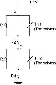
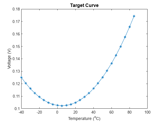
電圧源はポイント A を 1.1V に保持します。問題は、ポイント B の電圧が温度の関数としての目標曲線と一致するように、標準コンポーネントのリストから抵抗器とサーミスタを選択することです。

Tdata = -40:5:85;
Vdata = 1.026E-1 + -1.125E-4 * Tdata + 1.125E-5 * Tdata.^2;
plot(Tdata,Vdata,'-*');
title('Target Curve','FontSize',12); 
xlabel('Temperature (^oC)'); ylabel('Voltage (V)')

Figure contains an axes object. The axes object with title Target Curve, xlabel Temperature ( toThePowerOf o baseline C ), ylabel Voltage (V) contains an object of type line.

標準コンポーネントリストを読み込みます。

load StandardComponentValues

Res ベクトルには標準抵抗値が含まれています。ThBeta および ThVal ベクトルには、サーミスタの標準パラメーターが含まれています。サーミスタ抵抗の温度関数 $T$ は

$R_{T h} = \frac{R_{25}}{\exp (β \frac{T - T_{25}}{T \cdot T_{25}})} .$

$R_{T h}$ はサーミスタ抵抗です。
$R_{25}$ は 25 ℃ での抵抗、パラメーターThVal です。
$T_{25}$ は気温 25 度です。
$T$ は現在の温度です。
$β$ はサーミスタパラメーターThBeta です。

標準電圧計算に基づくと、 $R_{1} - T h_{1}$ ブロックの抵抗の等価直列抵抗値は

$R_{1}^{e q u i v a l e n t} = \frac{R_{1} {T h}_{1}}{R_{1} + {T h}_{1}}$ ,

そして $R_{3} - T h_{2}$ ブロックの等価抵抗は

$R_{3}^{e q u i v a l e n t} = \frac{R_{3} {T h}_{2}}{R_{3} + {T h}_{2}}$ .

したがって、B点の電圧は

$V = 1.1 \frac{R_{3}^{e q u i v a l e n t} + R_{4}}{R_{1}^{e q u i v a l e n t} + R_{2} + R_{3}^{e q u i v a l e n t} + R_{4}}$ .

問題をコードに変換する

問題は、電圧 $V$ が目標曲線に最もよく一致するように、抵抗器 $R_{1}$ から $R_{4}$ とサーミスタ $T h_{1}$ および $T h_{2}$ を選択することです。制御変数 x が次の値を表すようにします。

x(i) = $R_{i}$ のインデックス、i は 1 から 4 まで
x(5) = $T h_{1}$ のインデックス
x(6) = $T h_{2}$ のインデックス

tempCompCurve 関数は、結果の電圧を x と温度 Tdata に基づいて計算します。

type tempCompCurve

function F = tempCompCurve(x,Tdata)
%% Calculate Temperature Curve given Resistor and Thermistor Values
% Copyright (c) 2012-2019, MathWorks, Inc.
%% Input voltage
Vin = 1.1;

%% Thermistor Calculations
% Values in x: R1 R2 R3 R4 RTH1(T_25degc) Beta1 RTH2(T_25degc) Beta2
% Thermistors are represented by:
%   Room temperature is 25degc: T_25
%   Standard value is at 25degc: RTHx_25
%   RTHx is the thermistor resistance at various temperatures
% RTH(T) = RTH(T_25degc) / exp (Beta * (T-T_25)/(T*T_25))
T_25 = 298.15;
T_off = 273.15;
Beta1 = x(6);
Beta2 = x(8);
RTH1 = x(5) ./ exp(Beta1 * ((Tdata+T_off)-T_25)./((Tdata+T_off)*T_25));
RTH2 = x(7) ./ exp(Beta2 * ((Tdata+T_off)-T_25)./((Tdata+T_off)*T_25));

%% Define equivalent circuits for parallel Rs and RTHs
R1_eq = x(1)*RTH1./(x(1)+RTH1);
R3_eq = x(3)*RTH2./(x(3)+RTH2);

%% Calculate voltages at Point B
F = Vin * (R3_eq + x(4))./(R1_eq + x(2) + R3_eq + x(4));

目的関数は、目標温度範囲における、抵抗器とサーミスタのセットの目標曲線と結果として生じる電圧の差の二乗の合計です。

type objectiveFunction

function G = objectiveFunction(x,StdRes, StdTherm_Val, StdTherm_Beta,Tdata,Vdata)
%% Objective function for the thermistor problem
% Copyright (c) 2012-2019, MathWorks, Inc.

% % StdRes = vector of resistor values
% StdTherm_val = vector of nominal thermistor resistances
% StdTherm_Beta = vector of thermistor temperature coefficients

% Extract component values from tables using integers in x as indices
y = zeros(8,1);
x = round(x); % in case of noninteger components
y(1) = StdRes(x(1));
y(2) = StdRes(x(2));
y(3) = StdRes(x(3));
y(4) = StdRes(x(4));
y(5) = StdTherm_Val(x(5));
y(6) = StdTherm_Beta(x(5));
y(7) = StdTherm_Val(x(6));
y(8) = StdTherm_Beta(x(6));

% Calculate temperature curve for a particular set of components
F = tempCompCurve(y, Tdata);

% Compare simulated results to target curve
Residual = F(:) - Vdata(:);
Residual = Residual(1:2:26);
%%
G = Residual'*Residual; % sum of squares

進行状況の監視

最適化の進行状況を観察するには、これまでに見つかったシステムの最適な応答とターゲット曲線をプロットする出力関数を呼び出します。SurrOptimPlot 関数はこれらの曲線をプロットし、現在の目的関数の値が減少した場合にのみ曲線を更新します。このカスタム出力関数は長いため、ここでは示されていません。この出力関数の内容を表示するには、「type SurrOptimPlot」と入力します。

最適化問題

目的関数を最適化するには、整数変数を受け入れる surrogateopt を使用します。まず、すべての変数を整数に設定します。

intCon = 1:6;

すべての変数の下限を 1 に設定します。

lb = ones(1,6);

抵抗器の上限はすべて同じです。上限を Res データのエントリ数に設定します。

ub = length(Res)*ones(1,6);

サーミスタの上限を ThBeta データのエントリ数に設定します。

ub(5:6) = length(ThBeta)*[1,1];

SurrOptimPlot カスタム出力関数を使用し、プロット関数を使用しないオプションを設定します。また、最適化の中断を防ぐために、'checkfile.mat' という名前のチェックポイントファイルを指定します。

options = optimoptions('surrogateopt','CheckpointFile','C:\TEMP\checkfile.mat','PlotFcn',[],...
    'OutputFcn',@(a1,a2,a3)SurrOptimPlot(a1,a2,a3,Tdata,Vdata,Res,ThVal,ThBeta));

アルゴリズムに探索するポイントの初期セットをより適切に提供するには、デフォルトよりも大きな初期ランダムサンプルを指定します。

options.MinSurrogatePoints = 50;

最適化を実行します。

rng default % For reproducibility
objconstr = @(x)objectiveFunction(x,Res,ThVal,ThBeta,Tdata,Vdata);
[xOpt,Fval] = surrogateopt(objconstr,lb,ub,intCon,options);

Figure contains an axes object. The axes object with title Thermistor Network Temperature Curve, xlabel Temperature ( toThePowerOf o baseline C ), ylabel Voltage (V) contains 2 objects of type line. These objects represent Ideal Curve, surrogateopt Solution.

surrogateopt stopped because it exceeded the function evaluation limit set by 
'options.MaxFunctionEvaluations'.

より多くの関数評価による最適化

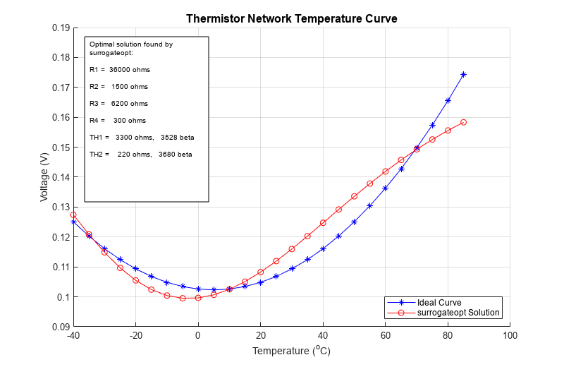
より良い適合を得るには、チェックポイントファイルから最適化を再開し、より多くの関数評価を指定します。今回は、surrogateoptplot プロット関数を使用して、最適化プロセスをより詳しく監視します。

clf % Clear previous figure
opts = optimoptions(options,'MaxFunctionEvaluations',600,'PlotFcn','surrogateoptplot');
[xOpt,Fval] = surrogateopt('C:\TEMP\checkfile.mat',opts);

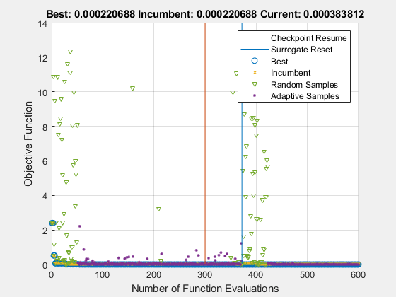
surrogateopt stopped because it exceeded the function evaluation limit set by 
'options.MaxFunctionEvaluations'.

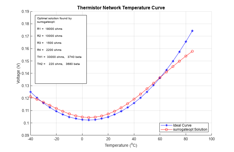
関数評価をさらに使用すると、適合性がわずかに向上します。

参考文献

[1] Lyon, Craig K. Genetic algorithm solves thermistor-network component values.EDN Network, March 19, 2008.https://www.edn.com/genetic-algorithm-solves-thermistor-network-component-values/ から入手可能。

参考

surrogateopt

トピック

サロゲート最適化

surrogateoptを使用した最適なコンポーネントの選択