fitSmithWilson

Fit the Smith-Wilson model to observed bond prices

Since R2024a

Syntax

outCurve = fitSmithWilson(Settle,Instruments,CleanPrice,UltimateForwardRate,LastLiquidPoint)

outCurve = fitSmithWilson(___Name=Value)

Description

outCurve = fitSmithWilson(Settle,Instruments,CleanPrice,UltimateForwardRate,LastLiquidPoint) fits a Smith-Wilson curve to observed bond prices and returns a parametercurve object.. After creating a parametercurve object for outCurve, you can use the associated object functions discountfactors, zerorates, and forwardrates.

outCurve = fitSmithWilson(___Name=Value) specifies options using one or more name-value arguments in addition to the input arguments in the previous syntax.

Examples

Fit Smith-Wilson Model to Bond Market Data

Define the bond data and use fininstrument to create a FixedBond instrument object.

Settle = datetime("15-Jun-2023");
Maturity = Settle + calyears([2 4 6 9 18 30]');
CleanPrice = [100.1;100.1;100.8;96.6;103.3;96.3];
CouponRate = [0.0400;0.0425;0.0450;0.0400;0.0500;0.0425];
Bonds = fininstrument("FixedBond",Maturity=Maturity,CouponRate=CouponRate)

Bonds=6×1 FixedBond array with properties:
    CouponRate
    Period
    Basis
    EndMonthRule
    Principal
    DaycountAdjustedCashFlow
    BusinessDayConvention
    Holidays
    IssueDate
    FirstCouponDate
    LastCouponDate
    StartDate
    Maturity
    Name

Use fitSmithWilson to create a parametercurve object.

UltimateForwardRate = .042;
LastLiquidPoint = 20;
SW = fitSmithWilson(Settle,Bonds,CleanPrice,UltimateForwardRate,LastLiquidPoint,Basis=4)

SW = 
  parametercurve with properties:

              Type: "discount"
            Settle: 15-Jun-2023
       Compounding: -1
             Basis: 4
    FunctionHandle: @(t)W(u_cf,t(:)')'*CF'*zeta+exp(-ultFwdInt*t(:))
        Parameters: 0.1317

You can use the parametercurve object (SW) to compute discountfactors, zerorates, and forwardrates.

outDiscountFactors=discountfactors(SW,[datetime("15-Jun-2024");datetime("15-Jun-2027")])

outDiscountFactors = 2×1

    0.9627
    0.8456

outZeroRates = zerorates(SW,[datetime("15-Jun-2024");datetime("15-Jun-2027")])

outZeroRates = 2×1

    0.0380
    0.0419

outForwardRates = forwardrates(SW,datetime("15-Jun-2024"),datetime("15-Jun-2027"))

outForwardRates = 
0.0432

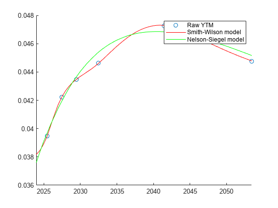
Compare Fit for Smith-Wilson Model and Nelson-Siegel Model to Bond Market Data

Define the bond market data and use bndyield to compute the raw yield to maturity.

Settle = datetime("15-Jun-2023");
Maturity = Settle + calyears([2 4 6 9 18 30]');
CleanPrice = [100.1;100.1;100.8;96.6;103.3;96.3];
CouponRate = [0.0400;0.0425;0.0450;0.0400;0.0500;0.0425];

YTM = bndyield(CleanPrice,CouponRate,Settle,Maturity)

YTM = 6×1

    0.0395
    0.0422
    0.0435
    0.0446
    0.0473
    0.0448

scatter(Maturity,YTM)

Use fininstrument to create a FixedBond instrument object using the bond data.

Bonds = fininstrument("FixedBond",Maturity=Maturity,CouponRate=CouponRate);

Use fitSmithWilson to create a parametercurve object.

UltimateForwardRate = .033;
LastLiquidPoint = 20;
SW = fitSmithWilson(Settle,Bonds,CleanPrice,UltimateForwardRate,LastLiquidPoint)

SW = 
  parametercurve with properties:

              Type: "discount"
            Settle: 15-Jun-2023
       Compounding: -1
             Basis: 3
    FunctionHandle: @(t)W(u_cf,t(:)')'*CF'*zeta+exp(-ultFwdInt*t(:))
        Parameters: 0.0613

Use fitNelsonSiegel to create a parametercurve object.

NS = fitNelsonSiegel(Settle, Bonds, CleanPrice)

Local minimum possible.

lsqnonlin stopped because the final change in the sum of squares relative to 
its initial value is less than the value of the function tolerance.

<stopping criteria details>

NS = 
  parametercurve with properties:

              Type: "zero"
            Settle: 15-Jun-2023
       Compounding: -1
             Basis: 0
    FunctionHandle: @(t)fitF(Params,t)
        Parameters: [6.7223e-08 0.0363 0.0904 16.5171]

Plot a comparison of the fit of a Smith-Wilson model to a Nelson-Siegel model for the bond market data.

hold on
PlottingTimes = calmonths(6:6:12*30)';
PlottingDates = Settle + PlottingTimes;
PY_SW = zero2pyld(zerorates(SW,PlottingDates),PlottingDates,Settle,'InputCompounding',-1,'InputBasis',3,'OutputCompounding',2);
PY_NS = zero2pyld(zerorates(NS,PlottingDates),PlottingDates,Settle,'InputCompounding',-1,'InputBasis',3,'OutputCompounding',2);
plot(PlottingDates,PY_SW,'r')
plot(PlottingDates,PY_NS,'g')
legend(["Raw YTM","Smith-Wilson model","Nelson-Siegel model"])

Input Arguments

Settle — Settlement date

datetime scalar | string scalar | date character vector

Settlement date, specified as a scalar datetime, string, or date character vector.

Data Types: datetime | string | char

Instruments — Bond instrument objects

scalar | array

Bond instrument objects, specified as a scalar bond object or an array of bond instruments objects using FixedBond.

Data Types: object

CleanPrice — Observed market prices

vector

Observed market prices, specified as a vector.

Data Types: double

UltimateForwardRate — Long-term constant forward rate

numeric

Long-term constant forward rate, specified as a numeric.

Data Types: double

LastLiquidPoint — Point on yield curve beyond which there is insufficient liquidity to value cash flows accurately

numeric

Point on the yield curve beyond which there is insufficient liquidity to value cash flows accurately, specified as a numeric.

Data Types: double

Name-Value Arguments

Specify optional pairs of arguments as Name1=Value1,...,NameN=ValueN, where Name is the argument name and Value is the corresponding value. Name-value arguments must appear after other arguments, but the order of the pairs does not matter.

Example: outCurve = fitSmithWilson(Settle,Bonds,CleanPrice,UltimateForwardRate,LastLiquidPoint,Basis=4,alpha=0.05)

Basis — Day count basis

0 (actual/actual) (default) | integer from 0 to 13

Day count basis, specified as Basis and a scalar integer.

• 0 — actual/actual

• 1 — 30/360 (SIA)

• 2 — actual/360

• 3 — actual/365

• 4 — 30/360 (PSA)

• 5 — 30/360 (ISDA)

• 6 — 30/360 (European)

• 7 — actual/365 (Japanese)

• 8 — actual/actual (ICMA)

• 9 — actual/360 (ICMA)

• 10 — actual/365 (ICMA)

• 11 — 30/360E (ICMA)

• 12 — actual/365 (ISDA)

• 13 — BUS/252

For more information, see Basis.

Data Types: double

alpha — Alpha value represents level of smoothness or flexibility of the yield curve

[] (default) | numeric between 0 and 1

Alpha value represents level of smoothness or flexibility of the yield curve, specified as alpha and a scalar numeric between 0 and 1.

The alpha value controls the tradeoff between fitting the observed market data and ensuring a smooth and plausible yield curve. By adjusting the alpha value, you can calibrate the Smith-Wilson model to different market conditions and risk preferences. A higher alpha value results in a smoother yield curve, while a lower alpha value allows for more flexibility and responsiveness to market movements.

Note

If you specify alpha, then fitSmithWilson ignores the input argument for LastLiquidPoint.

Data Types: double

Output Arguments

outCurve — Fitted Smith-Wilson model

parametercurve object

Fitted Smith-Wilson model, returned as a parametercurve object.

More About

Smith-Wilson Model

The Smith-Wilson model is a technique used to estimate the yield curve for discounting future cash flows.

The Smith-Wilson model is designed to handle long-dated liabilities and to accurately reflect the term structure of interest rates, particularly at the long end of the yield curve where market data is sparse. It uses a combination of market data and an ultimate forward rate (UFR) to extrapolate the yield curve to longer maturities.

Given the discount factor for tenor t, the Smith-Wilson equation to fit N prices for zero-coupon bonds with tenors u₁,...u_N, is

$$\begin{array}{l}P(t):=e^{-wt}+{\displaystyle \sum _{j=1}^N{\varsigma }_{j}W(t,u_{j),t}\ge 0,}\\ \text{where }w:=\log (1+UFR),\\ W(t,u_j):=e^{-w(t+u_j)}\left(\alpha (t\wedge u_j)-e^{-\alpha (t\vee u_{j)}}\sinh (\alpha (t\wedge u_j))\right)\end{array}$$

where:

• UFR is the ultimate forward rate.

• ɑ is a parameter determining the rate of convergence to the UFR.

References

[1] Lagerås A., and M. Lindholm. "Issues with Smith-Wilson Method." Insurance: Mathematics and Economics. Vol. 71, 2016, pp. 93–102.

[2] Smith, A., and T. Wilson. "Fitting Yield Curves with Long Term Constraints." Research report, Bacon and Woodrow, 2000.

Version History

Introduced in R2024a