Specify Regression Model with SARIMA Errors
This example shows how to specify a regression model with multiplicative seasonal ARIMA errors.
Load the Airline data set from the MATLAB® root folder, and load the recession data set. Plot the monthly passenger totals and log-totals.
load Data_Airline.mat
load Data_Recessions

y = DataTimeTable.PSSG;
logY = log(y);

figure
tiledlayout(2,1)
nexttile
plot(DataTimeTable.Time,y)
title('{\bf Monthly Passenger Totals (Jan1949 - Dec1960)}')
nexttile
plot(DataTimeTable.Time,log(y))
title('{\bf Monthly Passenger Log-Totals (Jan1949 - Dec1960)}')
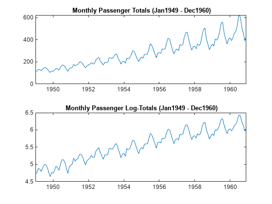
The log transformation seems to linearize the time series.
Construct this predictor, which is whether the country was in a recession during the sampled period. 0 means the country was not in a recession, and 1 means that it was in a recession.
X = zeros(numel(dates),1); % Preallocation
for j = 1:size(Recessions,1)
    X(dates >= Recessions(j,1) & dates <= Recessions(j,2)) = 1;
end
Fit the simple linear regression model,
to the data.
EstMdl = fitlm(X,logY);
Fit is a LinearModel that contains the least squares estimates.
Perform a residual diagnosis by plotting the residuals several ways.
figure
tiledlayout(2,2)
nexttile
plotResiduals(EstMdl,'caseorder','ResidualType','Standardized',...
    'LineStyle','-','MarkerSize',0.5)
nexttile
plotResiduals(EstMdl,'lagged','ResidualType','Standardized')
nexttile
plotResiduals(EstMdl,'probability','ResidualType','Standardized')
nexttile
plotResiduals(EstMdl,'histogram','ResidualType','Standardized')

r = EstMdl.Residuals.Standardized;

figure
tiledlayout(2,1)
nexttile
autocorr(r)
nexttile
parcorr(r)
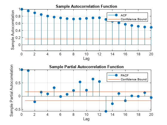
The residual plots indicate that the residuals are autocorrelated. The probability plot and histogram seem to indicate that the residuals are Gaussian.
The ACF of the residuals confirms that they are autocorrelated.
Take the 1st difference of the residuals and plot the ACF and PACF of the differenced residuals.
dR = diff(r);

figure
tiledlayout(2,1)
nexttile
autocorr(dR,'NumLags',50)
nexttile
parcorr(dR,'NumLags',50)
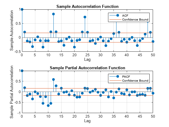
The ACF shows that there are significantly large autocorrelations, particularly at every 12th lag. This indicates that the residuals have 12th degree seasonal integration.
Take the first and 12th differences of the residuals. Plot the differenced residuals, and their ACF and PACF.
DiffPoly = LagOp([1 -1]);
SDiffPoly = LagOp([1 -1],'Lags',[0, 12]);
diffR = filter(DiffPoly*SDiffPoly,r);

figure
tiledlayout("flow")
nexttile([1 2])
plot(diffR)
axis tight
nexttile
autocorr(diffR)
h = gca;
h.FontSize = 7;
nexttile
parcorr(diffR)
h = gca;
h.FontSize = 7;
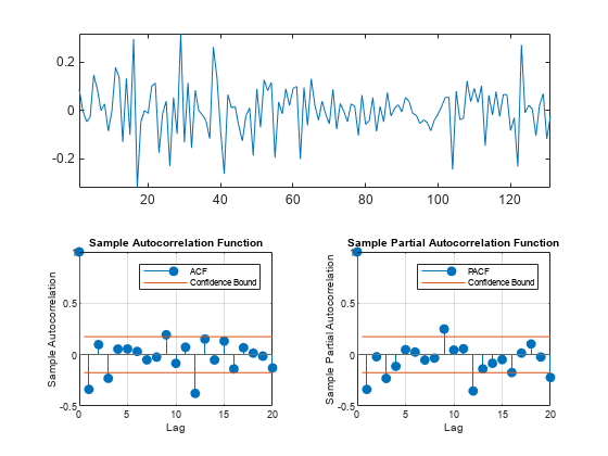
The residuals resemble white noise (with possible heteroscedasticity). According to Box and Jenkins (1994), Chapter 9, the ACF and PACF indicate that the unconditional disturbances are an model.
Specify the regression model with errors:
Mdl = regARIMA('MALags',1,'D',1,'Seasonality',12,'SMALags',12)
Mdl =
  regARIMA with properties:

     Description: "ARIMA(0,1,1) Error Model Seasonally Integrated with Seasonal MA(12) (Gaussian Distribution)"
      SeriesName: "Y"
    Distribution: Name = "Gaussian"
       Intercept: NaN
            Beta: [1×0]
               P: 13
               D: 1
               Q: 13
              AR: {}
             SAR: {}
              MA: {NaN} at lag [1]
             SMA: {NaN} at lag [12]
     Seasonality: 12
        Variance: NaN
Mdl is a regression model with errors. By default, the innovations are Gaussian, and all parameters are NaN. The property:
P= p + D + + s = 0 + 1 + 0 + 12 = 13.Q= q + = 1 + 12 = 13.
Therefore, the software requires at least 13 presample observations to initialize the model.
Pass Mdl, y, and X into estimate to estimate the model. In order to simulate or forecast responses using simulate or forecast, you need to set values to all parameters.
References:
Box, G. E. P., G. M. Jenkins, and G. C. Reinsel. Time Series Analysis: Forecasting and Control. 3rd ed. Englewood Cliffs, NJ: Prentice Hall, 1994.
See Also
regARIMA | estimate | simulate | forecast | LinearModel
Topics
- Create Regression Models with ARIMA Errors
- Specify Default Regression Model with ARIMA Errors
- Create Regression Models with AR Errors
- Create Regression Models with MA Errors
- Create Regression Models with ARMA Errors
- Create Regression Models with SARIMA Errors
- Specify ARIMA Error Model Innovation Distribution